The ability to accurately model and interpret complex data sets is paramount. This technical exploration delves into three sophisticated modelling techniques:

• Polynomial Models,
• Fractional Polynomials, and
• Spline Models.

Each of these models serves as a fundamental tool in the statistical toolkit, enabling us to capture and understand the intricacies of linear and non-linear relationships inherent in real-world data.

As a bio-statistician entrenched in the technical aspects of data analysis, I recognize the critical importance of these models. We will commence with an examination of Polynomial Models, discussing their mathematical underpinnings and practical applications in capturing curvilinear trends. Next, we will navigate through the Fractional Polynomials, a more flexible extension of traditional polynomials, adept at modelling asymmetric patterns. Lastly, we will explore Spline Models, one of the most flexible approach in data fitting, capable of adapting to complex and segmented patterns in data.

This post is designed not just to inform but to provide a technical understanding of these models with examples, illustrating their relevance and application in contemporary data analysis. Whether you are a data scientist, a statistician, or a researcher grappling with complex data sets, this exploration aims to enhance the modelling arsenal, offering insights into when and how to apply these models effectively.

Polynomial Models

Polynomial Models, represented by functions of the form

are foundational in modelling curvilinear relationships. In this formulation, each $a_i$ (where $i = 0, 1, \ldots, n$) denotes the coefficient corresponding to the $i$-th term of the polynomial, and $x$ is the independent or exploratory variable. The degree $n$ of the polynomial determines the model’s complexity, with higher degrees allowing for more intricate curve shapes.

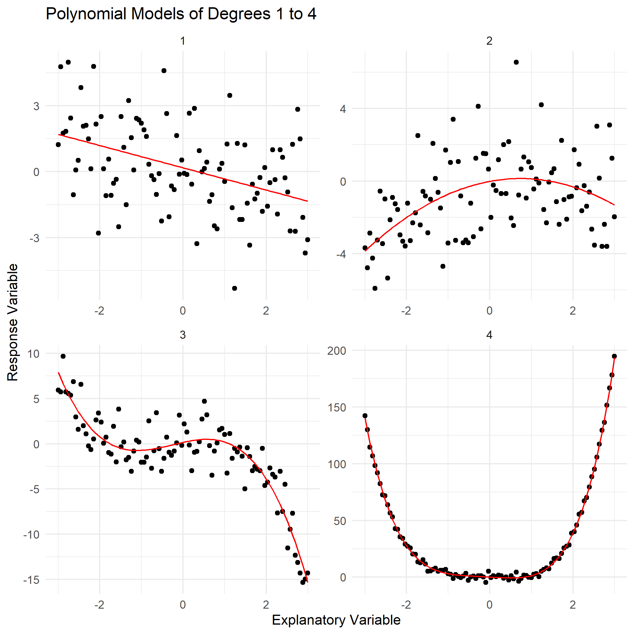
These models are particularly useful in capturing the non-linear dynamics often observed in real-world data. For instance, a quadratic model (where $n = 2$) can describe simple parabolic trends, while higher-degree models, such as cubic ($n = 3$) or quartic ($n = 4$), enable the representation of more complex and varied behaviours (Figure 1).

Comparative Visualization of Polynomial Fits: Degrees 1 to 4

However, increasing the degree $n$ also increases the risk of overfitting, a phenomenon where the model adapts too closely to the specificities of the training data, including noise, at the expense of generalizability to new data (Figure 2). Overfitting leads to models that perform poorly in predictive scenarios, failing to capture the true underlying trend.

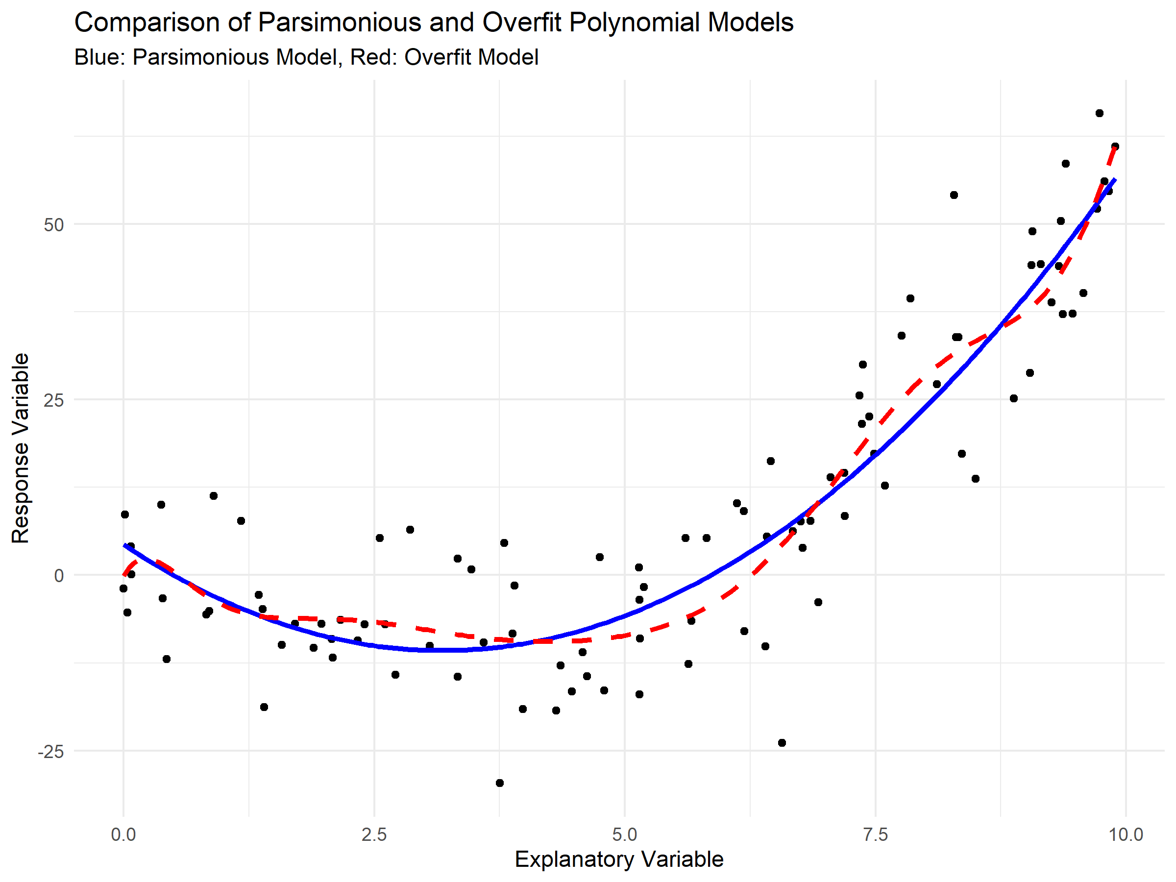
Visualizing Model Complexity: Parsimonious vs Overfit Polynomial Fits

Polynomial models are extensively applied across various disciplines. In physics, they are instrumental in modelling motion under uniform acceleration, among other phenomena. In economics, polynomial trends are fitted to time series data to understand market dynamics. In biological sciences, these models aid in interpreting growth rates and simple gene expression patterns. 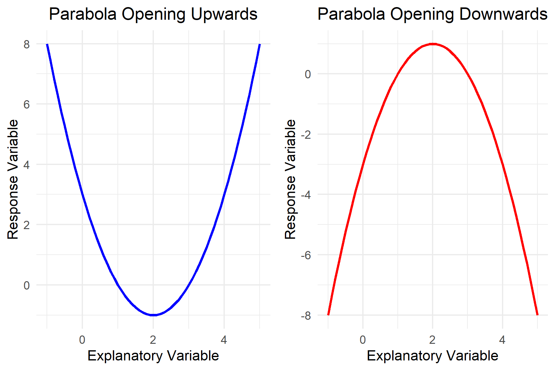The interpretation of the coefficients $a_i$ can provide significant insights; for instance, in the quadratic model $y = ax^2 + bx + c$, the sign of $a$ determines the direction in which the parabola opens, offering crucial information about the nature of the relationship being modelled (Figure 3).

Parabola Opening Upwards and Downwards

In practical applications, the selection of the polynomial degree $n$ is critical. It is a balance between capturing the complexity of the data and avoiding overfitting (Figure 2). Techniques such as cross-validation, where the data is divided into training and testing sets, can be used to determine the optimal degree of the polynomial. Additionally, statistical measures like the Akaike Information Criterion (AIC) or the Bayesian Information Criterion (BIC) are often employed to select the most appropriate model by balancing model fit and complexity.

In summary, Polynomial Models are a versatile and powerful tool in statistical modelling. Their ability to approximate complex functions with a relatively straightforward mathematical formulation makes them a fundamental component in various fields of data analysis.

While traditional polynomial models are highly effective, they sometimes lack the flexibility required for certain types of data, particularly those exhibiting asymmetric trends. This limitation led to the development of fractional polynomial models, which extend the concept of polynomial models by allowing for fractional exponents. This advancement provides a greater ability to fit a wider range of curves and is especially useful in cases where the relationship between variables is not adequately captured by integer exponents.

Fractional Polynomial Models

Fractional Polynomials represent an advanced evolution of traditional polynomial models, marked by their use of non-integer, real-number exponents in the independent variable. Mathematically, they are expressed as

where $x$ is the independent variable, $\beta_i$ are coefficients, and $p_i$ are the variable powers. These powers, unlike the integer-only powers in traditional polynomials, can include any real number like $0.5$, $-1$, or $2.3$. This flexibility significantly broadens the modeling capability of polynomials, allowing for more precise fitting to complex and asymmetric data patterns. Terms such as $x^{-1}$ and $x^{0.5}$, representing the reciprocal and square root of $x$ respectively, enable the modeling of relationships that exhibit dramatic changes over different ranges of $x$, a task challenging for standard polynomial models with integer exponents.

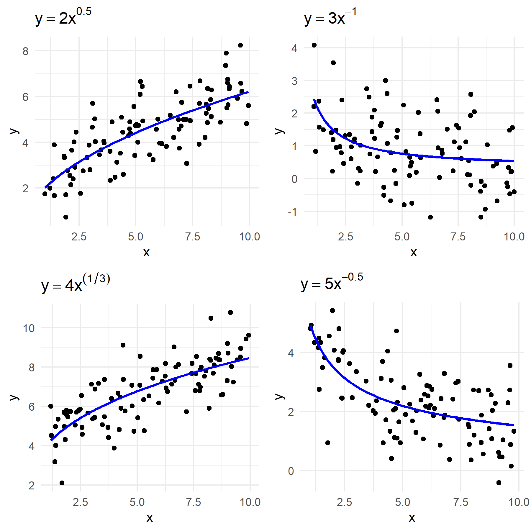
Comparative Visualization of Fractional Polynomial Fits

The utility of fractional polynomials extends to various fields, notably in medical statistics and biological data analysis, where data patterns often defy symmetry. They are particularly adept in modeling phenomena like dose-response curves in pharmacokinetics and progression rates of diseases, where the response changes in a non-linear fashion. Such flexibility makes them invaluable in scenarios where data exhibit complex, non-standard behaviors.

However, the complexity of fractional polynomials can pose interpretational challenges, and like their traditional counterparts, they are susceptible to overfitting. This risk is heightened with the inclusion of multiple fractional terms or higher degrees, necessitating careful model selection and validation processes. Methods such as cross-validation or the use of information criteria like AIC or BIC are often employed to balance model fit against the risk of overfitting.

Finding Optimal Power Values in Fractional Polynomials

The process of finding the best values for $p_1, p_2, \ldots, p_n$ is inherently iterative and may require a combination of statistical testing, validation techniques, and expert judgement. The goal is to have a balance between a model that fits the data well, is not overly complex, and is robust to variations in model parameters.

In Figure 5, I exemplify this process by fitting various fractional polynomial models to the dataset. Through the application of the Bayesian Information Criterion (BIC), I identified the most parsimonious model, which is succinctly expressed mathematically as

and the corresponding BIC value for this model is denoted as $−144.34$.

Comparative Visualization of Fractional Polynomial Fits

Below I have described some possible approaches to achieve this objective:

Initial Power Selection: Start with a set of candidate powers, often including a mix of positive, negative, and fractional values. Common choices are \(-2, -1, -0.5, 0, 0.5, 1, 2, 3\). The selection of these initial powers is guided by prior knowledge about the data, theoretical considerations, or exploratory analysis.

Model Fitting and Comparison: Fit fractional polynomial models using different combinations of these candidate powers. This fitting can be done using least squares regression or other suitable methods depending on the nature of the data. For each model, compute a goodness-of-fit statistic, such as the residual sum of squares (RSS) or the Akaike Information Criterion (AIC).

Iterative Testing: Employ an iterative approach to test various combinations of powers. This might involve starting with a simple model and gradually adding complexity (increasing the number of terms) while monitoring the improvement in the fit.

Cross-Validation: To guard against overfitting, especially in models with higher degrees or more terms, use cross-validation. Divide your data into training and testing sets. Fit the model to the training set and evaluate its performance on the testing set. This step helps in assessing the model’s predictive accuracy.

Statistical Significance: Assess the statistical significance of the coefficients associated with each term in the model. Non-significant terms might suggest that certain powers do not contribute meaningfully to the model and could be excluded.

Model Selection Criteria: Use model selection criteria like AIC or BIC to compare models with different combinations of powers. These criteria balance the goodness of fit with the complexity of the model, helping to choose a model that is both accurate and parsimonious.

Sensitivity Analysis: Conduct sensitivity analyses by varying the powers slightly to see how robust the model is to changes in these parameters. This step is crucial to understand the stability and reliability of the model.

While fractional polynomials offer enhanced modelling flexibility over traditional polynomials, they sometimes fall short in handling data with distinct behavioural changes across different segments. This limitation summed to the difficulty in determine $p_i$ are where spline models come into play. Spline models, constructed as piecewise polynomials, provide localized fitting capabilities, adapting seamlessly to variations within different data segments. Such adaptability is particularly useful in datasets with distinct phases or regimes. Thus, spline models emerge as a natural progression when fractional polynomials alone are insufficient to model the intricate patterns present in the data

Spline Models

Splines are a class of mathematical functions used in statistical modeling, defined as piecewise polynomials that are joined at specific points called knots. Mathematically, if we denote a spline function by $S(x)$, it can be represented as:

where $P_i(x)$ are polynomial functions of degree $d$, typically represented as

for each piece of the spline, with $a_{i0}, a_{i1}, \ldots, a_{id}$ being the coefficients that vary from one segment of the spline to another. The knots $k_1, k_2, \ldots, k_{n-1}$ are specific values in the domain of $x$ where these polynomial pieces meet. Splines ensure continuity and smoothness at these knots by enforcing that both the function and its derivatives up to degree $d-1$ are continuous across the knots. This mathematical formulation allows splines to flexibly model a wide range of functions by varying the number and position of the knots as well as the degree of the polynomial pieces.

Splines, with their diverse forms, can have a variety of applications, each type distinguished by its unique features and mathematical formulation. Linear splines represent the most basic form, where each segment $P_i(x)$ is a linear function, typically $P_i(x) = a_{i0} + a_{i1}x$. These are straightforward to compute and are used in applications requiring simple, piecewise linear approximations.

Cubic splines elevate the complexity and smoothness, with each $P_i(x)$ being a third-degree polynomial:

. Their widespread adoption is attributed to their ability to model smooth, continuous curves, making them highly suitable for applications in curve fitting, computer-aided design, and modelling non-linear relationships in data.

B-splines, or basis splines, while they can also be cubic, offer a more general and flexible approach. They are defined not by the splines themselves, but by a set of basis functions, which are piecewise polynomials of a specified degree. The key advantage of B-splines is their local control; adjustments in one part of the spline affect only a limited region around that part. This is due to their basis functions having minimal support, which means each function is non-zero only over a small interval.

For B-splines, the mathematical representation shifts from individual polynomial pieces to a sum of basis functions, each weighted by a coefficient. These basis functions are defined over the knots and have local support. The B-spline representation can be expressed as:

Here, $B_{i,d}(x)$ are the B-spline basis functions of degree $d$, and $c_i$ are the coefficients. The basis functions $B_{i,d}(x)$ are defined recursively, starting with degree 0 (piecewise constant functions) and building up to the desired degree. The recursive definition for a B-spline basis function of degree $d$ is given by:

The knots $k_0, k_1, \ldots, k_{n+d}$ in the case of B-splines extend beyond the range of the data to ensure that the spline is well-defined at the boundaries. This expansion of the knot sequence provides a framework for the B-spline basis functions to cover the entire domain of the data. Unlike traditional splines, where each polynomial piece is defined explicitly, B-splines construct the spline function as a linear combination of these basis functions, providing a high degree of flexibility and local control over the shape of the spline. This formulation allows for efficient computation and adjustments in a localized manner, making B-splines a powerful tool for modelling complex data in various applications.

Example

Figure 6 visualizes the fitting of four distinct statistical models to a dataset:

• a cubic polynomial,
• a fractional polynomial,
• a cubic spline, and
• a B-spline.

The explanatory variable is shown along the x-axis, while the response variable is on the y-axis.

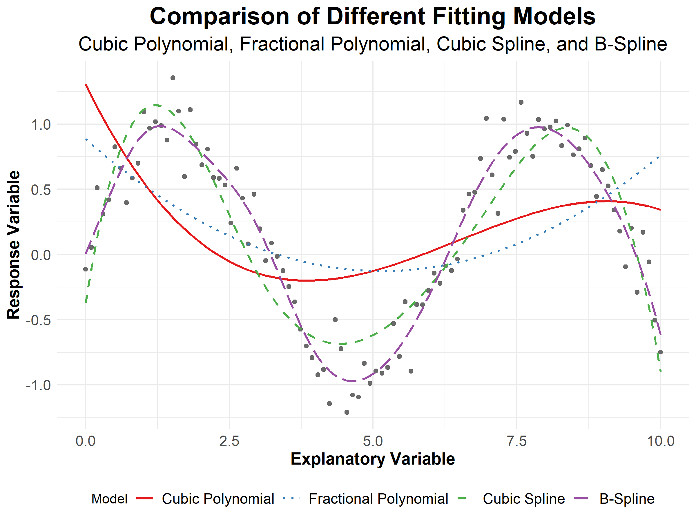
Comparison of Different Fitting Models

The plot provides a comparative visualization of four distinct statistical models applied to the same data set, with the cubic polynomial model (solid red line) demonstrating a poor fit. It captures the global tendency but lacks the intricacy to model local data variations, likely due to its restrictive assumption of a single global function without ‘breaks’. In contrast, the fractional polynomial (dotted blue line) incorporates power transformations of the explanatory variable, allowing for a more flexible functional form and better accommodation of non-linear relationships within the data. Nevertheless, it continues to apply a global approach to the data, which is evidently insufficient for modelling the localized fluctuations observed in the dataset. Both models underperform, suggesting that their global fitting strategies are inadequate for datasets. A more complex polynomial might offer an enhanced fit, but at the risk of overfitting, which must be judiciously managed.

More nuanced fits are achieved with the spline-based models. The cubic spline (dashed green line) employs piecewise third-degree polynomials, joining at the knots—strategically placed along the domain of the explanatory variable—to enhance model flexibility. This allows the cubic spline to conform more closely to the data’s local variations and structural shifts. The B-spline model (long-dashed purple line), with its basis function approach, offers a superior level of smoothness and local control, manifesting in its ability to trace the dataset’s oscillatory pattern with considerable precision.

The visual assessment thus underscores the critical role of model selection in statistical analysis, emphasizing that the appropriateness of a model is contingent upon its alignment with the data’s inherent patterns and the analysis objectives. The choice of model has profound implications for the accuracy of predictions and the robustness of inferences drawn from the data.

Challenges

The primary challenge in using spline models lies in the selection of knots. The number and location of knots significantly influence the model’s complexity and its ability to capture underlying patterns in data. Too few knots can lead to underfitting, while too many can cause overfitting. There is no universal method for optimal knot placement, often requiring a combination of data-driven techniques and expert judgement. Additionally, spline models can become computationally intensive with an increasing number of knots.

Splines are implemented through specialized algorithms that construct the piecewise polynomial functions and determine the appropriate knot positions, like in the R package splines. These algorithms often utilize basis functions, such as B-spline basis functions, which provide a stable and efficient way to represent spline curves. Computational techniques, like penalized least squares for smoothing splines, are employed to balance model fit and smoothness. Most statistical software packages offer built-in functions for spline modelling, simplifying their application in practical scenarios.

Selection Process for Spline Models

The selection process for spline models involves determining the optimal type and number of splines, along with the placement of knots, to best fit the data while avoiding overfitting. This process is a critical step in spline modelling and typically involves a blend of statistical techniques and domain expertise.

Type Selection: The first step is choosing the type of spline (e.g., linear, cubic, B-spline, smoothing spline). The choice depends on the nature of the data and the smoothness required in the model. For instance, cubic splines are often chosen for their balance between flexibility and smoothness.

Number of Knots: Deciding on the number of knots is crucial as it controls the flexibility of the spline model. As explained previously, fewer knots result in a smoother, but potentially underfit model, while more knots can capture finer details but risk overfitting. Methods like cross-validation can be used to determine an optimal number of knots (caret package in R). In cross-validation, the data is divided into subsets; the model is trained on some subsets and validated on others, with the goal of minimizing prediction error.

Knot Placement: The location of knots is equally important. Knots can be placed at quantiles of the independent variable, which is a common strategy for evenly distributing them across the range of data. Alternatively, adaptive methods can be used where knot placement is data-driven, focusing on regions where the function appears to change rapidly.

Model Complexity and Regularization: For smoothing splines, the degree of smoothness is controlled by a smoothing parameter. Techniques like the Akaike Information Criterion (AIC), Bayesian Information Criterion (BIC), or generalized cross-validation (GCV) are used to select this parameter. These methods aim to find a balance between the goodness of fit and the complexity of the model.

Model Validation: After selecting the spline model, it is validated using unseen data or through resampling methods like bootstrapping. This step is crucial to ensure that the model generalizes well and does not merely capture the idiosyncrasies of the training data.

Citation

1. For attribution, please cite this work as:

2. BibTeX citation

@misc{oliveira2024polynomials,
  author = {Oliveira, Thiago},
  title = {Exploring Polynomial, Fractional Polynomial, and Spline Models},
  year = {2024}
}

Did you find this page helpful? Consider sharing it 🙌