1 Pearson correlation as a starting point
2 Different questions about dependence
3 Linear association and the Gaussian case
4 Monotonic but nonlinear relationships
5 Dependence with zero linear correlation
6 Directional dependence
7 Sensitivity to the observed sample
- 7.1 Influential observations
- 7.2 Range restriction
8 Marginal and partial correlation
9 Final remarks
10 References
11 Reproducibility

1 Pearson correlation as a starting point

If someone asks for the correlation between two continuous variables, the default answer is usually Pearson’s correlation coefficient. It is familiar, interpretable and closely connected to linear regression. Given two variables \(X\) and \(Y\),

\[ \rho_{XY} = \frac{\operatorname{Cov}(X,Y)}{\sigma_X\sigma_Y}. \]

Its question is precise.

To what extent do \(X\) and \(Y\) vary together linearly?

The figure below shows several different data generating mechanisms. Pearson’s \(r\) ranges from about 0.61 to 0.78. All five coefficients indicate positive linear association, but the scatterplots show substantial differences in curvature, conditional spread, group structure and influential observations.

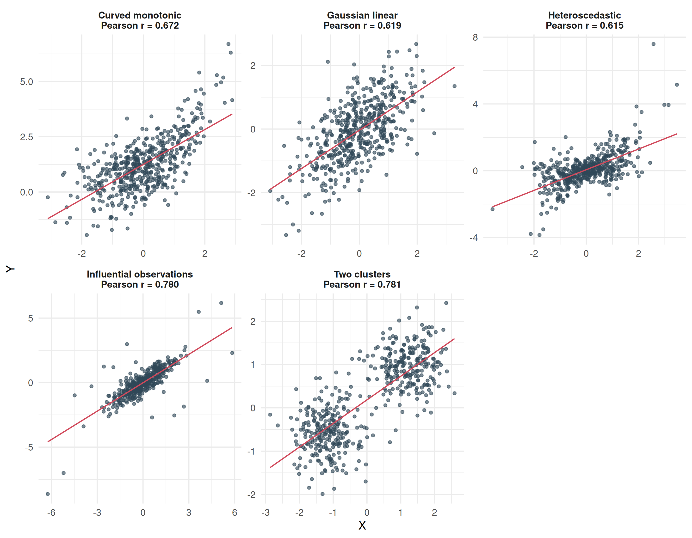
Pearson compresses the joint distribution into a summary of second moments. To make this precise, suppose both variables have finite, nonzero variances. Write \(\mu_X=E(X)\) and \(\mu_Y=E(Y)\), and define the standardised variables \(Z_X=(X-\mu_X)/\sigma_X\) and \(Z_Y=(Y-\mu_Y)/\sigma_Y\). Then

\[ \rho_{XY} = \frac{E(XY)-\mu_X\mu_Y}{\sigma_X\sigma_Y} = E(Z_XZ_Y). \]

The means, variances and mixed second moment \(E(XY)\) are the only features of the joint distribution entering this calculation. Here \(\sigma_X^2=E(X^2)-\mu_X^2\), and similarly for \(Y\). Different joint distributions can share all these moments and therefore have exactly the same Pearson correlation. The sample coefficient \(r\) is the analogous normalised sum of centred products.

Example with identical moments

Let \(X\) take the values \(-1\), \(0\) and \(1\), each with probability \(1/3\). Compare two ways to generate \(Y\).

Dependent pair. Set \(Y=X^2\). The three equally likely pairs are \((-1,1)\), \((0,0)\) and \((1,1)\).
Independent pair. Draw \(Y\) independently of \(X\), with \(P(Y=1)=2/3\) and \(P(Y=0)=1/3\).

Both constructions give exactly the same marginal distributions for \(X\) and \(Y\), so their marginal means and variances are identical. They also have the same mixed second moment. For the dependent pair,

\[ E(XY)=\frac{(-1)(1)+(0)(0)+(1)(1)}{3}=0. \]

For the independent pair, \(E(XY)=E(X)E(Y)=0\), because \(E(X)=0\). Thus both have zero covariance and Pearson correlation zero.

The difference is easy to see. In the dependent pair, knowing \(X\) tells us \(Y\) exactly. In the independent pair, knowing \(X\) does not change the probabilities of \(Y\). Their moments agree, but their joint distributions do not.

Pearson cannot by itself tell us whether the conditional mean is curved, whether conditional variance changes with \(X\), whether the population contains distinct groups, or whether a few observations exert unusual influence.

The heteroscedastic panel illustrates the conditional variance issue. Similar \(r\) can accompany very different \(\operatorname{Var}(Y\mid X)\), as the following population example makes explicit.

Example of heteroscedasticity

Let \(X\), \(\varepsilon_1\) and \(\varepsilon_2\) be independent standard normal variables. Compare

\[ Y_1=X+\varepsilon_1, \qquad Y_2=X+X\varepsilon_2. \]

Both have the same conditional mean, \(E(Y_1\mid X)=E(Y_2\mid X)=X\). Their conditional variances differ.

\[ \operatorname{Var}(Y_1\mid X)=1, \qquad \operatorname{Var}(Y_2\mid X)=X^2. \]

The first relationship has constant vertical spread. The second is tight near \(X=0\) and becomes more variable as \(|X|\) increases.

Nevertheless, both have \(\operatorname{Cov}(X,Y_i)=1\). By the law of total variance,

\[ \operatorname{Var}(Y_i) =\operatorname{Var}\{E(Y_i\mid X)\} +E\{\operatorname{Var}(Y_i\mid X)\} =1+1=2, \qquad i=1,2. \]

For \(Y_2\), the second term is \(E(X^2)=1\). Hence the two population Pearson correlations are exactly equal.

\[ \rho_{X,Y_1}=\rho_{X,Y_2}=\frac{1}{\sqrt{2}}\approx 0.707. \]

The simulations below use fixed seeds and moderately sized samples. Each introduces a feature of dependence that the preceding summaries leave unresolved.

2 Different questions about dependence

The measures correspond to different statistical questions.

Statistical question	Measure
Do \(X\) and \(Y\) vary together linearly?	Pearson correlation
Do larger values of one variable tend to correspond monotonically to larger or smaller values of the other?	Spearman correlation
Do pairs of observations tend to preserve the same ordering?	Kendall’s \(\tau\)
Is there dependence, including nonlinear or nonmonotonic dependence?	Distance correlation
Is there dependence detectable through flexible kernel representations?	HSIC
How strongly does \(Y\) depend on \(X\), allowing the two directions to differ?	Chatterjee’s \(\xi\)
Does the apparent association persist when unusual observations have limited influence?	Robust correlation estimators
Does linear association remain after adjusting for other variables?	Partial correlation

For this article, I use the following organisation as a teaching device rather than as a formal taxonomy.

Questions about dependence
|
+-- Linear association
|   +-- Pearson
|
+-- Monotonic ordering
|   +-- Spearman
|   +-- Kendall
|
+-- General dependence
|   +-- Distance correlation
|   +-- HSIC
|
+-- Directional dependence
|   +-- Chatterjee's xi
|
+-- Sensitivity to observations
|   +-- Robust correlations
|
+-- Conditional association
    +-- Partial correlation

3 Linear association and the Gaussian case

Pearson is closely linked to linear regression. In ordinary simple linear regression with an intercept, \(r^2 = R^2\). This is one reason Pearson correlation is such a natural summary when the relationship is genuinely linear.

Pearson is invariant to changes of location and scale. If we add constants or multiply both variables by positive constants, \(r\) does not change. Multiplying one variable by a negative constant reverses the sign.

To calibrate the measures against a known population model, start with a jointly Gaussian pair with a specified Pearson correlation. We use the construction

\[ X \sim N(0,1), \qquad Y = \rho X + \sqrt{1-\rho^2}\varepsilon, \]

where \(\varepsilon\sim N(0,1)\) is independent of \(X\), and we set \(\rho=0.7\).

The coefficients are chosen to keep both variables centred with unit variance. Independence gives

\[ \begin{aligned} \operatorname{Var}(Y)&=\rho^2+(1-\rho^2)=1,\\ \operatorname{Cov}(X,Y)&=\rho\operatorname{Var}(X)=\rho. \end{aligned} \]

As a linear combination of independent normal variables, \(Y\) has the marginal distribution

\[ Y\sim N\!\left(0,\rho^2+(1-\rho^2)\right)=N(0,1). \]

Since both standard deviations equal one, \(\operatorname{Cor}(X,Y)=\rho\). The factor \(\sqrt{1-\rho^2}\) scales the independent noise so that changing \(\rho\) changes the dependence while preserving the marginal variance. These assumptions define the calibration example; they require separate justification when modelling real data.

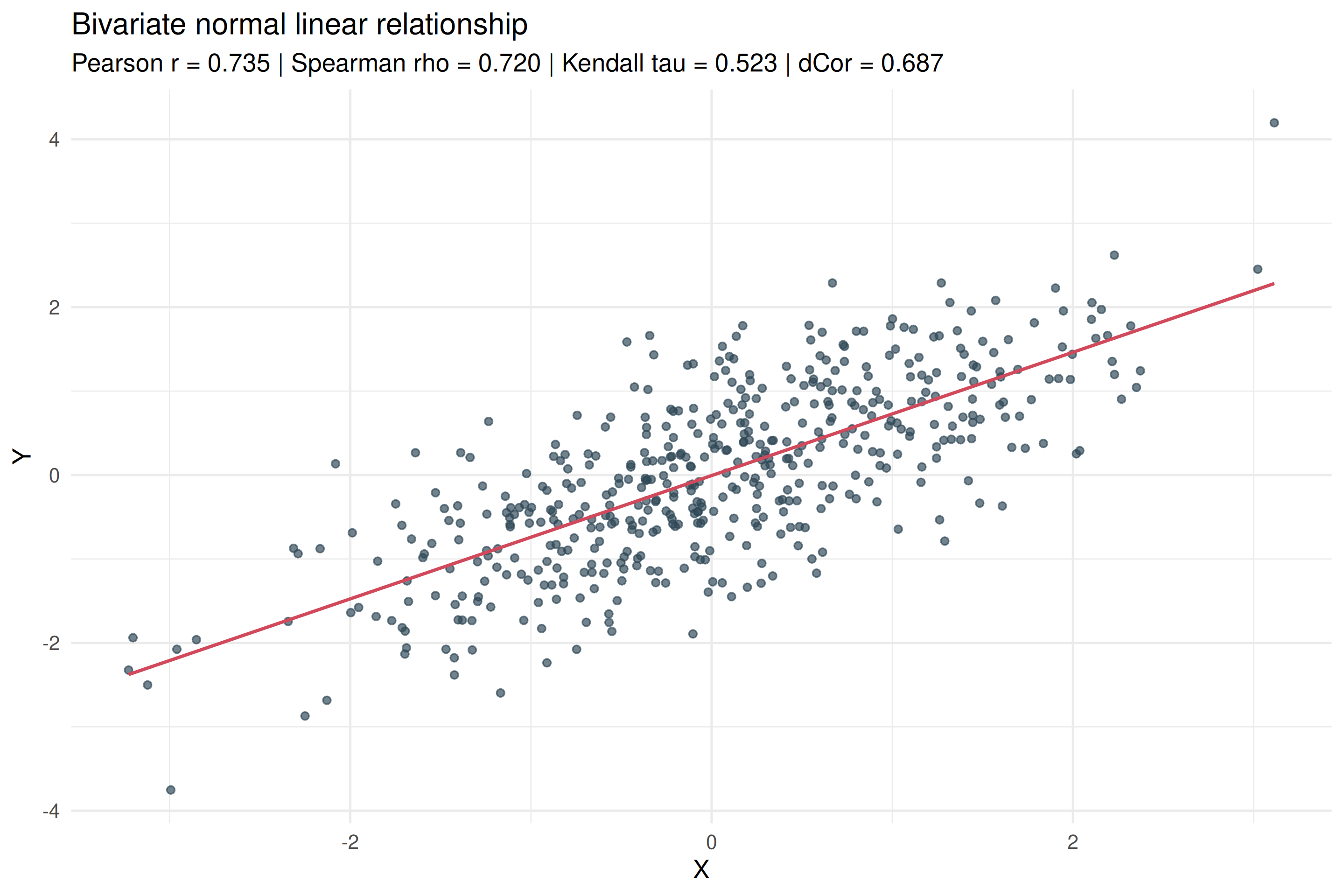
For this simulated sample, Pearson’s \(r\) is 0.735, compared with the generating population correlation \(\rho=0.7\). The difference reflects sampling variability.

To obtain the joint distribution, write the construction as a matrix transformation.

\[ \begin{pmatrix}X\\Y\end{pmatrix} =A\begin{pmatrix}X\\\varepsilon\end{pmatrix}, \qquad A=\begin{pmatrix} 1 & 0\\ \rho & \sqrt{1-\rho^2} \end{pmatrix}. \]

Independence gives \((X,\varepsilon)^{\mathsf T}\sim N_2(\mathbf{0},I_2)\). A linear transformation of a multivariate normal vector is also multivariate normal. Its mean vector is \(A\mathbf{0}=\mathbf{0}\) and its covariance matrix is

\[ AI_2A^{\mathsf T}=AA^{\mathsf T} =\begin{pmatrix} 1 & \rho\\ \rho & \rho^2+(1-\rho^2) \end{pmatrix} =\begin{pmatrix} 1 & \rho\\ \rho & 1 \end{pmatrix}. \]

Therefore,

\[ \begin{pmatrix} X \\ Y \end{pmatrix} \sim N_2 \left[ \begin{pmatrix} 0 \\ 0 \end{pmatrix}, \begin{pmatrix} 1 & \rho \\ \rho & 1 \end{pmatrix} \right]. \]

For this jointly Gaussian model,

\[ \rho = 0 \iff X \perp Y. \]

Under bivariate normality, means, variances and Pearson’s \(\rho\) determine the joint distribution. After standardisation, \(\rho\) is the single free dependence parameter. This requires joint normality; two variables can each be marginally normal without being jointly normal. The rank correlations are deterministic functions of \(\rho\) (de Winter, Gosling and Potter, 2016, equations 9 and 10).

\[ \tau=\frac{2}{\pi}\arcsin(\rho), \qquad \rho_S=\frac{6}{\pi}\arcsin\left(\frac{\rho}{2}\right). \]

Converting Gaussian correlation measures

For a bivariate normal population with Pearson correlation \(\rho=0.7\), the corresponding rank correlations are

\[ \begin{aligned} \tau&=\frac{2}{\pi}\arcsin(0.7)\approx 0.494,\\ \rho_S&=\frac{6}{\pi}\arcsin(0.7/2)\approx 0.683. \end{aligned} \]

The inverse functions recover Pearson correlation from either rank coefficient.

\[ \begin{aligned} \rho&=\sin\!\left(\frac{\pi\tau}{2}\right),\\ \rho&=2\sin\!\left(\frac{\pi\rho_S}{6}\right). \end{aligned} \]

Population distance correlation also has an exact Gaussian relation (Székely, Rizzo and Bakirov, 2007, Theorem 7).

\[ \operatorname{dCor}^2(X,Y)= \frac{ \rho\arcsin(\rho)+\sqrt{1-\rho^2} -\rho\arcsin(\rho/2)-\sqrt{4-\rho^2}+1 }{1+\pi/3-\sqrt{3}}. \]

Taking the nonnegative square root gives dCor. For \(\rho=0.7\), dCor is approximately 0.650. The same value results from \(\rho=-0.7\). Under this model, dCor determines \(|\rho|\) but cannot recover its sign.

The following R function accepts population Pearson, Spearman or Kendall correlation and returns all three plus population dCor. Applying these relations to sample coefficients imposes the Gaussian model and need not reproduce the other estimates from that sample. The converted dCor is a population model value, distinct from an empirical distance correlation.

gaussian_correlations <- function (value, from = c("pearson", "spearman", "kendall")) 
{
    from <- match.arg(from)
    if (!is.numeric(value) || length(value) == 0L || any(!is.finite(value)) || 
        any(abs(value) > 1)) {
        stop("value must contain finite numeric correlations between -1 and 1.", 
            call. = FALSE)
    }
    rho <- switch(from, pearson = value, spearman = 2 * sin(pi * value/6), kendall = sin(pi * 
        value/2))
    rho[abs(value) == 1] <- sign(value[abs(value) == 1])
    dcor_squared <- (rho * (asin(rho) - asin(rho/2)) + rho^2 * (1/(2 + sqrt(4 - 
        rho^2)) - 1/(1 + sqrt(1 - rho^2))))/(1 + pi/3 - sqrt(3))
    data.frame(pearson = rho, spearman = 6/pi * asin(rho/2), kendall = 2/pi * 
        asin(rho), dcor = sqrt(pmax(0, pmin(1, dcor_squared))))
}

For example, start from Pearson and then convert back from each rank coefficient using the unrounded values.

gaussian_example <- gaussian_correlations(0.7, from = "pearson")
gaussian_from_s <- gaussian_correlations(gaussian_example$spearman, from = "spearman")
gaussian_from_k <- gaussian_correlations(gaussian_example$kendall, from = "kendall")

Input	Pearson	Spearman	Kendall	dCor
Pearson	0.7	0.683	0.494	0.65
Spearman	0.7	0.683	0.494	0.65
Kendall	0.7	0.683	0.494	0.65

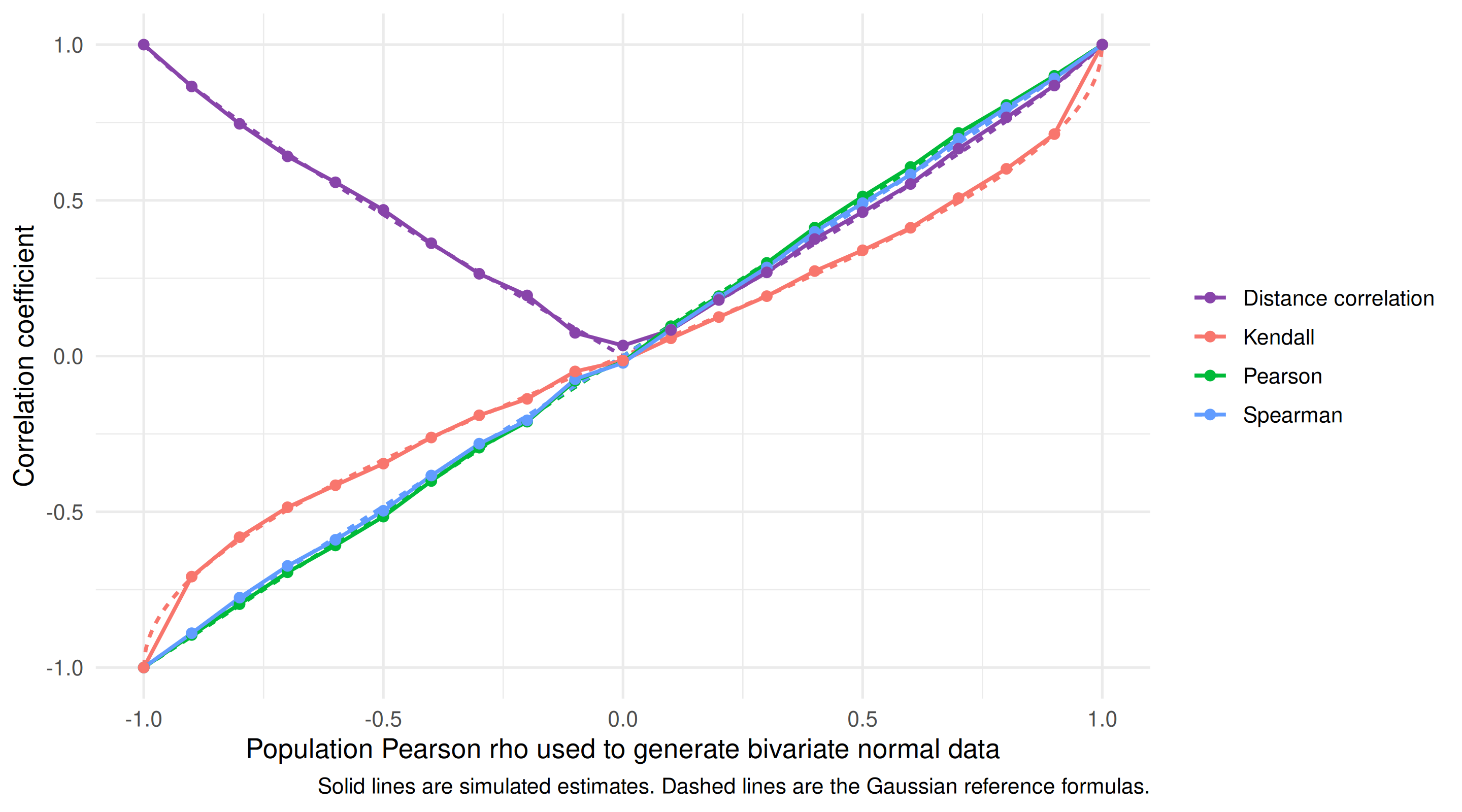
The next figure compares simulated estimates with their Gaussian reference curves across \(\rho\in[-1,1]\). The horizontal axis is the generating Pearson parameter. The signed coefficients range from \(-1\) to \(1\), whereas dCor reaches \(1\) at both endpoints and has a symmetric population curve with minimum zero at independence.

4 Monotonic but nonlinear relationships

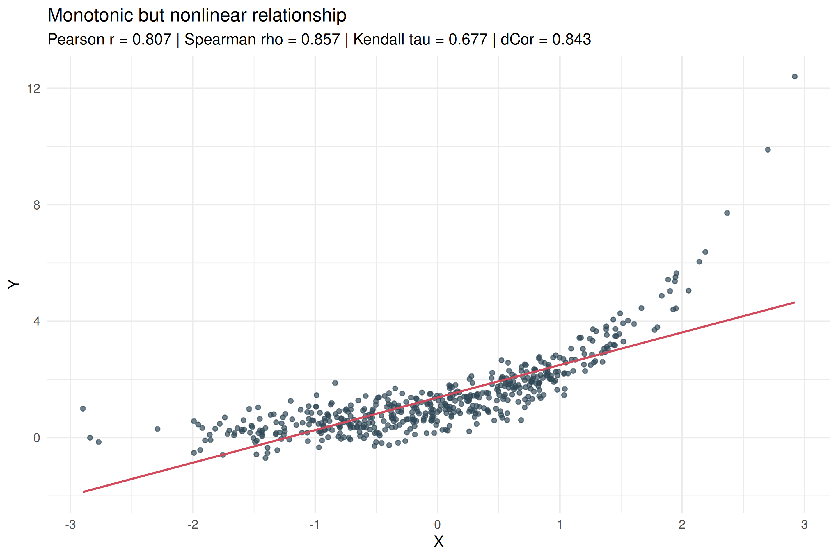
Now simulate a relationship that is clearly increasing but not straight.

\[ Y = \exp(aX) + \varepsilon. \]

An increasing function preserves order in the sense that

\[ x_1<x_2 \quad\Longrightarrow\quad g(x_1)\leq g(x_2). \]

For a strictly increasing function, \(x_1<x_2\Longrightarrow g(x_1)<g(x_2)\). When \(a>0\), \(g(x)=\exp(ax)\) is strictly increasing because \(g'(x)=a\exp(ax)>0\), but it is nonlinear. Monotonicity describes ordering, whereas linearity describes an affine form.

Without noise, a deterministic relationship \(Y=g(X)\) with \(g\) strictly increasing and continuous variables gives identical orderings of \(X\) and \(Y\). Consequently,

\[ \rho_S=1,\qquad \tau=1. \]

For Pearson, assuming finite, nonzero variances,

\[ |\rho_{XY}|=1 \quad\Longleftrightarrow\quad Y=\alpha+\beta X\ \text{almost surely},\qquad \beta\neq0. \]

The deterministic curve \(Y=\exp(X)\) is therefore perfectly monotonic without being perfectly linearly correlated, whenever Pearson correlation is defined for the continuous distribution of \(X\). In the simulation above, noise can reverse the ordering of individual observations, so the rank correlations need not equal one.

For continuous variables, population Spearman correlation is

\[ \rho_S =\operatorname{Cor}\{F_X(X),F_Y(Y)\} =12E\{F_X(X)F_Y(Y)\}-3. \]

The second equality follows because both marginal distribution transforms are uniform on \((0,1)\). In a sample,

\[ \hat\rho_S=\operatorname{Cor}\{R(X),R(Y)\}, \]

where \(R(X)\) and \(R(Y)\) are the sample ranks. Spearman’s correlation is Pearson correlation applied to ranks.

If \(g\) is strictly increasing, then, in the absence of ties,

\[ R\{g(X)\}=R(X), \qquad \rho_S\{g(X),Y\}=\rho_S(X,Y). \]

A strictly increasing transformation of either variable preserves Spearman correlation. A strictly decreasing transformation of one variable reverses its sign. This invariance does not extend to arbitrary nonlinear transformations. Spearman specifically measures monotonic rank association, rather than general nonlinear dependence.

Kendall compares the orderings of two independent copies \((X_1,Y_1)\) and \((X_2,Y_2)\). They are concordant when \((X_1-X_2)(Y_1-Y_2)>0\) and discordant when \((X_1-X_2)(Y_1-Y_2)<0\). For continuous variables without ties,

\[ \begin{aligned} \tau &=P(\text{concordant})-P(\text{discordant})\\ &=E\!\left[\operatorname{sign}\{(X_1-X_2)(Y_1-Y_2)\}\right]. \end{aligned} \]

Kendall’s \(\tau\) compares how often randomly selected pairs are ordered consistently in \(X\) and \(Y\) with how often the ordering is reversed.

Measure	What is compared?	Main feature
Pearson	Original values	Linear association
Spearman	Ranks	Monotonic association
Kendall	Pairwise concordance	Pairwise ordering

In this simulation, Pearson’s \(r=0.807\), Spearman’s \(\hat\rho_S=0.857\) and Kendall’s \(\hat\tau=0.677\). Spearman remains high, consistent with the strong monotonic ordering visible in the scatterplot, and positive Kendall indicates that concordant pairs are more frequent than discordant pairs. The curve and the coefficients together describe strong positive ordering despite the noise. Pearson and Spearman estimate different population functionals, so their numerical difference is not a direct measure of curvature.

Technical note on ties

Real data can contain ties because of rounding, ordinal scales or discrete measurements. In matrixCorr, Spearman uses average ranks, also called midranks, and Kendall uses \(\tau_b\) to adjust for ties, reducing to \(\tau_a\) when there are none. Chatterjee’s \(\xi\) has its own handling of response ties and an explicit rule for breaking ties in the sorting variable. The tie rule should be part of the analysis.

Strong dependence need not preserve ordering, as the quadratic example illustrates.

5 Dependence with zero linear correlation

The most important nonmonotonic example here is

\[ X \sim N(0,1), \qquad Y = X^2 + \varepsilon. \]

The simulated noise is independent of \(X\) and centred, so \(E(\varepsilon)=0\) and \(\varepsilon\perp X\). Because the standard normal distribution is symmetric,

\[ \operatorname{Cov}(X,X^2) = E(X^3)-E(X)E(X^2) = 0. \]

For the actual response,

\[ \begin{aligned} \operatorname{Cov}(X,Y) &=\operatorname{Cov}(X,X^2)+\operatorname{Cov}(X,\varepsilon)\\ &=0+0\\ &=0. \end{aligned} \]

Thus the population Pearson correlation is zero even though the conditional mean of \(Y\) varies with \(X\).

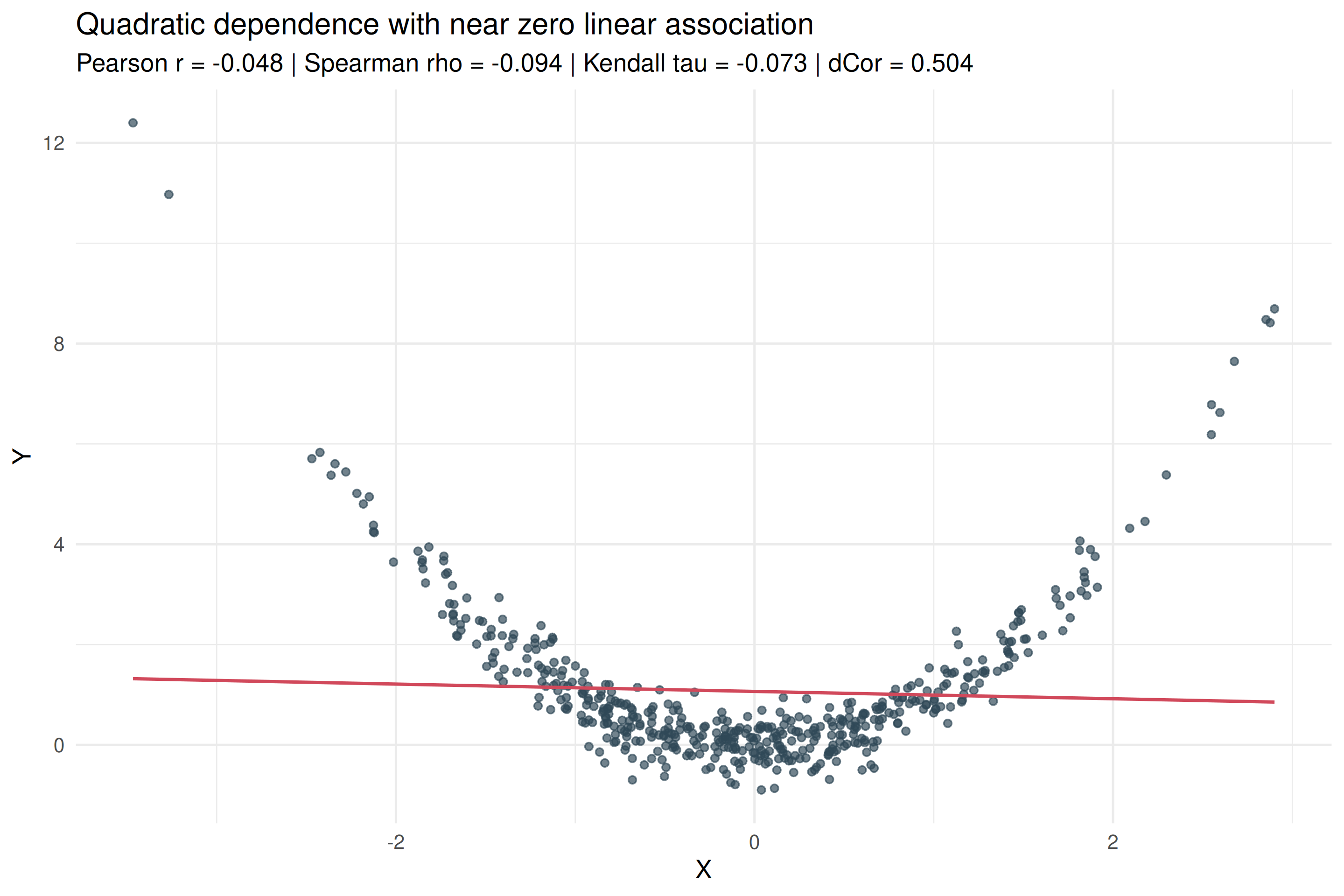
The curve bends back on itself. The increasing and decreasing branches cancel in the linear summary and do not give a consistent global rank ordering.

pearson	spearman	kendall	dcor	hsic	xi_y_given_x	xi_x_given_y
-0.048	-0.094	-0.073	0.504	0.366	0.589	0.15

Distance covariance compares patterns of pairwise distances. When \(E|X|<\infty\) and \(E|Y|<\infty\), population distance correlation satisfies (Székely, Rizzo and Bakirov, 2007)

\[ \operatorname{dCor}(X,Y)=0 \iff X\perp Y. \]

Kernel methods compare functions of \(X\) and \(Y\) rather than only their original values (Gretton, Herbrich et al., 2005). HSIC uses these kernel representations to measure dependence through a cross covariance operator (Gretton, Bousquet et al., 2005). With characteristic kernels such as the Gaussian RBF kernel, population HSIC is zero if and only if the variables are independent (Gretton et al., 2007; Sriperumbudur et al., 2010).

The tutorial uses Gaussian kernels, the median bandwidth rule, the biased empirical estimator and normalise = TRUE. Its HSIC values are therefore normalised kernel correlations. Unlike Pearson, there is no empirical HSIC number independent of the kernel and its tuning parameters. The specification is held fixed across scenarios, although the median rule adapts the numerical bandwidth to each sample. The software conventions for both measures are documented under Reproducibility.

Pearson, Spearman and Kendall can be positive or negative. Conventional dCor and the normalised HSIC measure used here are nonnegative and do not assign a global increasing or decreasing direction. Such a sign may have no useful global interpretation for a quadratic or periodic relationship.

The phenomenon is not specific to a quadratic relationship. Periodic dependence gives another example in which linear and rank summaries can be weak while general dependence remains clear.

\[ X \sim U(-\pi,\pi), \qquad Y = \sin(2X)+\varepsilon. \]

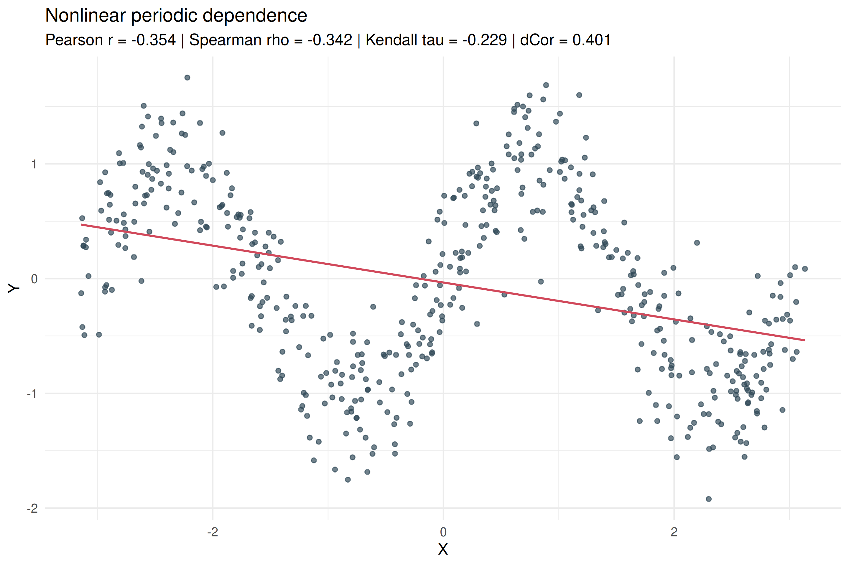
This periodic draw retains moderate negative linear and rank association (\(r = -0.354\) and \(\rho_S = -0.342\)). The scatterplot shows the oscillation that those summaries compress.

The panels below place the quadratic example alongside the linear, monotonic and periodic scenarios.

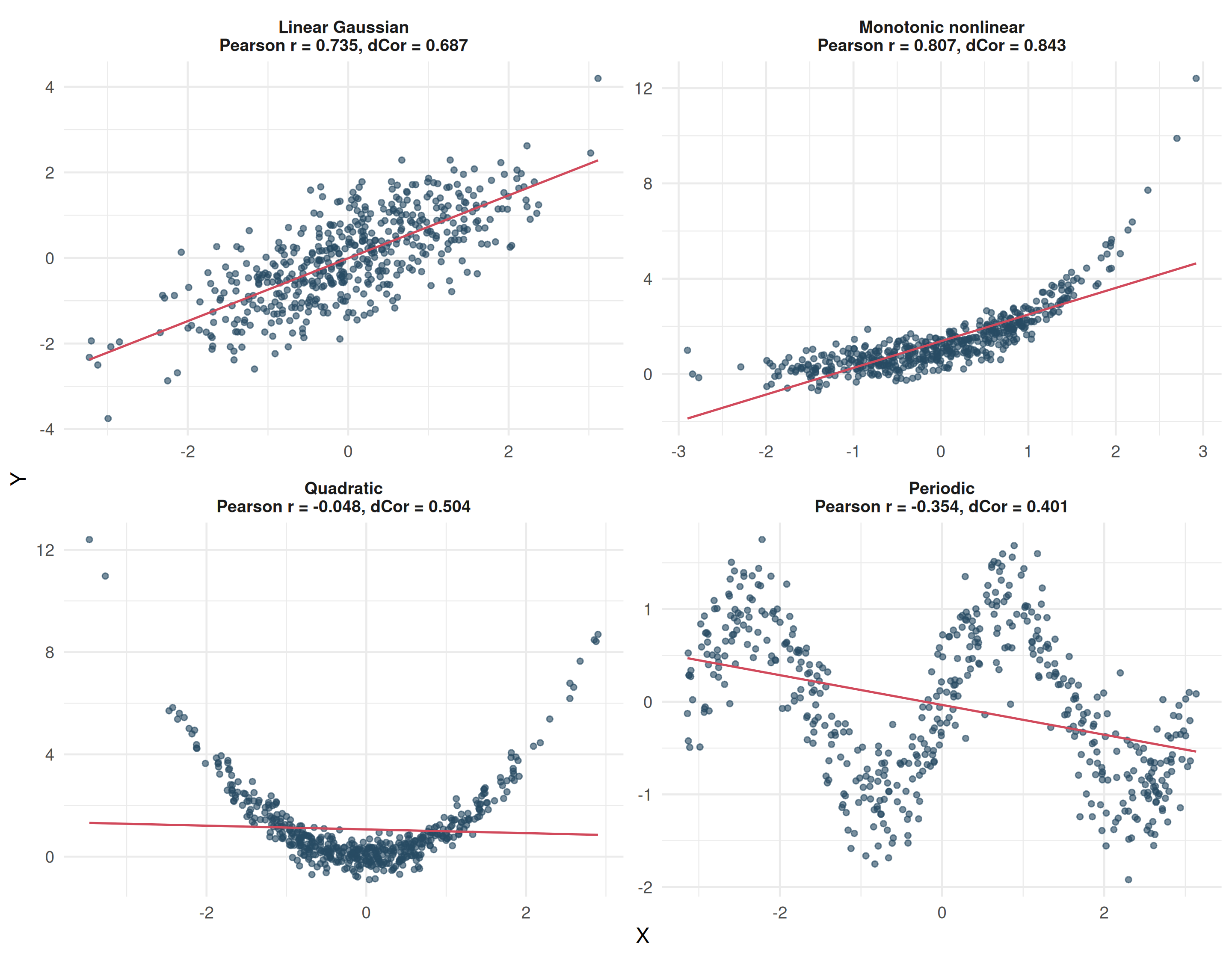
Distance correlation and HSIC address dependence rather than functional form. Detecting dependence still leaves subsequent modelling to explain its shape. In practice, I would use one of them when independence is the scientific question or when the plotted structure is inadequately described by linear and rank summaries. For an uncomplicated monotonic relationship, an additional general dependence coefficient may add little substantive information.

The preceding measures are symmetric in their arguments. We can also ask whether knowing \(X\) informs the distribution of \(Y\) in the same way that knowing \(Y\) informs the distribution of \(X\).

6 Directional dependence

Chatterjee’s \(\xi\) asks how much knowing one variable tells us about the other. The order matters. The call

xi_corr(x, y)

estimates \(\xi(x, y)\), where x is the sorting or predictor variable and y is the response or ranked variable. Read this as using x to learn about y.

For nondegenerate \(Y\), meaning that \(Y\) does not always take the same value, the population target is (Chatterjee, 2021, Theorem 1.1)

\[ \xi(X,Y)= \frac{ \int \operatorname{Var}\!\left[ E\{\mathbf{1}(Y\geq t)\mid X\} \right] \,dF_Y(t) }{ \int \operatorname{Var}\{\mathbf{1}(Y\geq t)\} \,dF_Y(t) }. \]

Read the equation as a collection of yes or no questions. Choose a cutoff \(t\) and ask whether \(Y\) is at least that large. The indicator \(\mathbf{1}(Y\geq t)\) is 1 when the answer is yes and 0 otherwise. Averaging these answers gives a probability. The conditional expectation \(E\{\mathbf{1}(Y\geq t)\mid X\}\), also written \(P(Y\geq t\mid X)\), is the chance of a yes answer when we know \(X\). The vertical bar means “given that we know”.

The top of the fraction measures how much this chance changes as \(X\) changes. Here \(\operatorname{Var}\) measures that spread. The bottom measures the spread in the original yes or no answers, providing a reference for the comparison. The integral signs mean that we average each kind of spread across cutoffs, weighted according to the distribution of \(Y\), denoted by \(F_Y\). The fraction compares these two averages, describing how much variation in the cutoff questions is explained by knowing \(X\).

The population coefficient lies between zero and one. Under independence, knowing \(X\) does not change the chance of a yes answer, so \(P(Y\geq t\mid X)=P(Y\geq t)\). The top of the fraction is zero and \(\xi(X,Y)=0\). At the other extreme, if \(Y=f(X)\) almost surely for a measurable \(f\), then knowing \(X\) fixes \(Y\) and settles every cutoff question. “Almost surely” means with probability one. The top and bottom are then equal, giving \(\xi(X,Y)=1\).

Reversing the order changes the question. When \(X\) is also nondegenerate, \(\xi(Y,X)\) uses knowledge of \(Y\) to ask whether \(X\) passes different cutoffs. Its probabilities are \(P(X\geq t\mid Y)\), averaged over the distribution of \(X\). Knowing \(X\) to explain \(Y\) and knowing \(Y\) to explain \(X\) need not be equally informative in this sense.

For the quadratic example without noise, \(Y=X^2\) is determined by \(X\). In the reverse direction, \(X=\pm\sqrt{Y}\), so knowledge of \(Y\) leaves the sign unresolved. Thus \(\xi(X,Y)=1\) and \(\xi(Y,X)<1\). The exact reverse population value is unnecessary for this comparison.

xi_y_given_x	xi_x_given_y	direction_confirmed
0.999	0.269	TRUE

This validation uses a random continuous sample so the reverse calculation is not driven by exact ties in \(Y=X^2\). It confirms the label used below. xi(X, Y) means “Y given X” in this article.

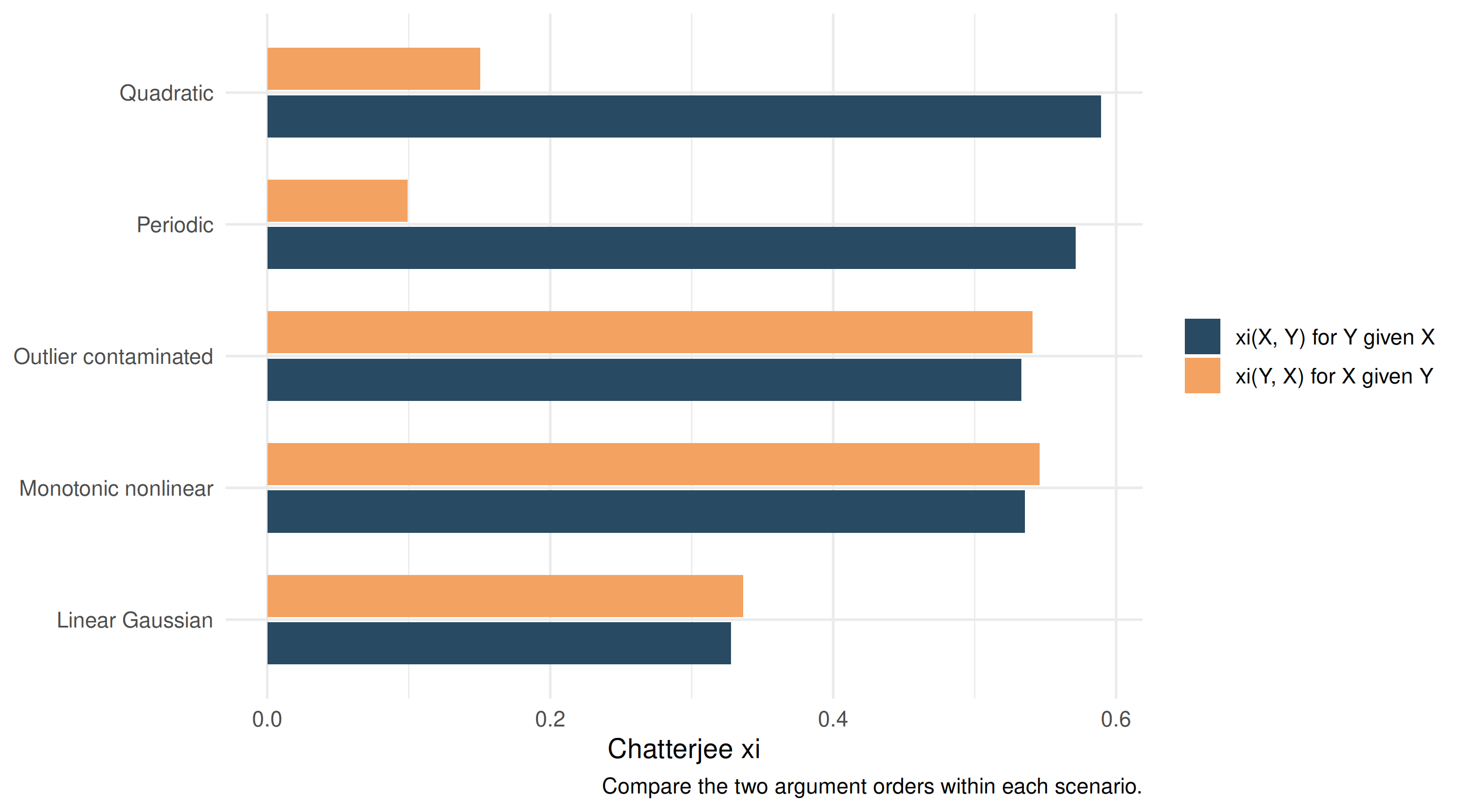
In practice, I would use \(\xi\) when it matters whether knowing \(X\) helps explain \(Y\) more than knowing \(Y\) helps explain \(X\). Threshold and saturation relationships, like the quadratic curve, can give the same response for several inputs.

If the relationship is roughly linear or monotonic and the scientific question treats both variables equally, Pearson, Spearman or Kendall may already give a more interpretable summary. I would add \(\xi\) when the difference between the two orders matters, rather than calculate it automatically.

Population pattern	Interpretation in the sense measured by \(\xi\)
\(\xi(X,Y)\approx\xi(Y,X)\)	Similar dependence strength in both directions
\(\xi(X,Y)>\xi(Y,X)\)	Stronger directional dependence of \(Y\) on \(X\) than of \(X\) on \(Y\)
\(\xi(X,Y)\) near zero	Knowing \(X\) explains little about the cutoff questions for \(Y\)
\(\xi(X,Y)\) near one	Knowing \(X\) explains most cutoff variation, without implying exact determinism

The guide describes population patterns, not formal classification rules. Directional dependence is not evidence of causal direction. Nor does it describe signed association. \(\xi(X,Y)\) can differ from \(\xi(Y,X)\) without indicating whether \(Y\) increases or decreases with \(X\).

\[ \text{directionality}\neq\text{sign}\neq\text{causality}. \]

The original finite sample statistic need not reach one even for an exact functional relationship. With continuous observations and no ties, its upper bound is \((n-2)/(n+1)\), which approaches one as the sample grows (Dalitz, Arning and Goebbels, 2024). It can also be negative in finite samples; that does not indicate decreasing association. The optional software rescaling is described under Reproducibility.

Chatterjee’s original statistic can have low local power against some alternatives (Shi, Drton and Han, 2022). Modified rank statistics can improve this aspect when independence testing is the primary objective (Lin and Han, 2023).

The next examples hold the underlying regression mechanism fixed and change which observations enter the sample.

7 Sensitivity to the observed sample

7.1 Influential observations

We deliberately move 4% of observations from a positive linear relationship into positions with high leverage opposing the main trend. This adversarial contamination exposes the influence of a small subset of the sample.

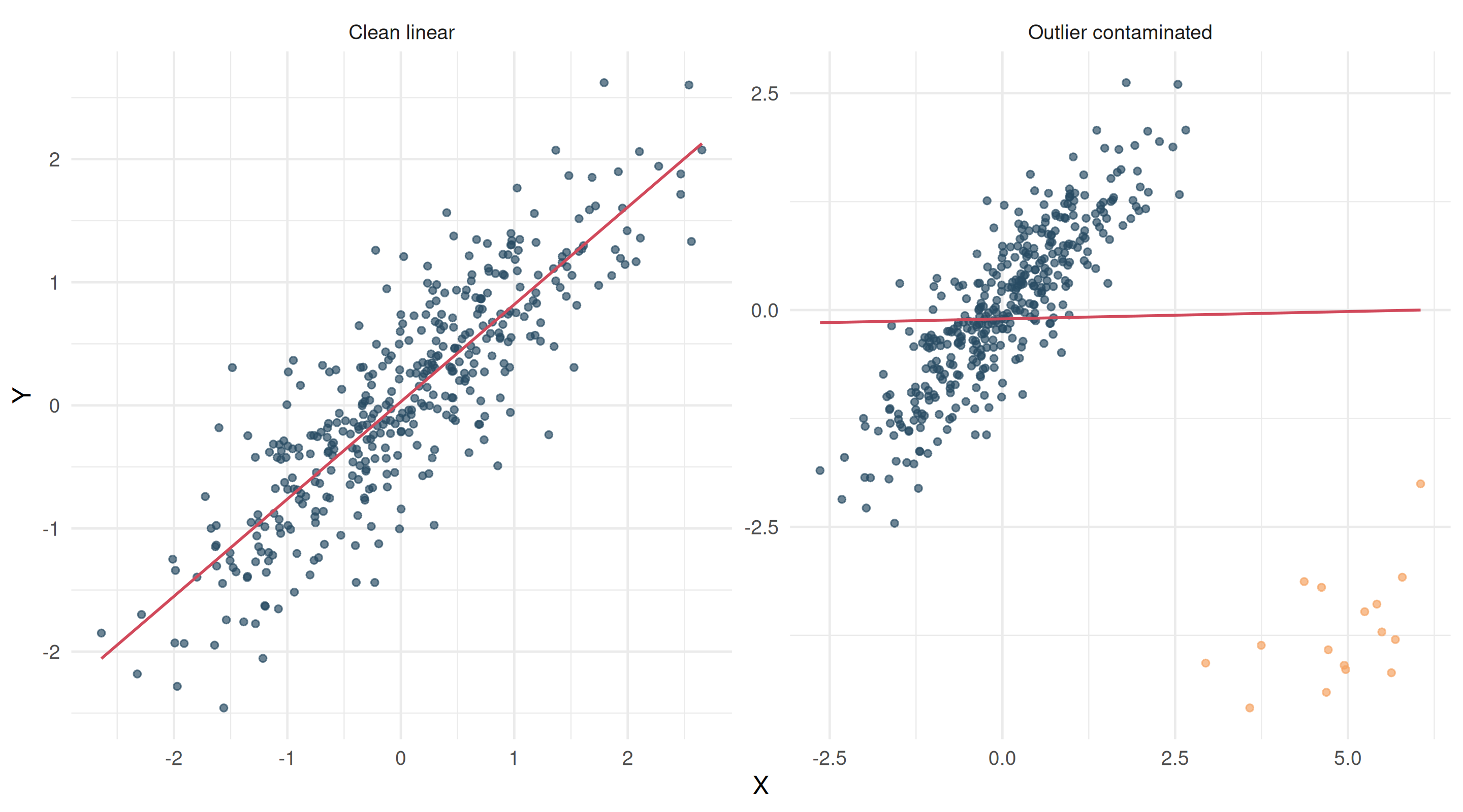
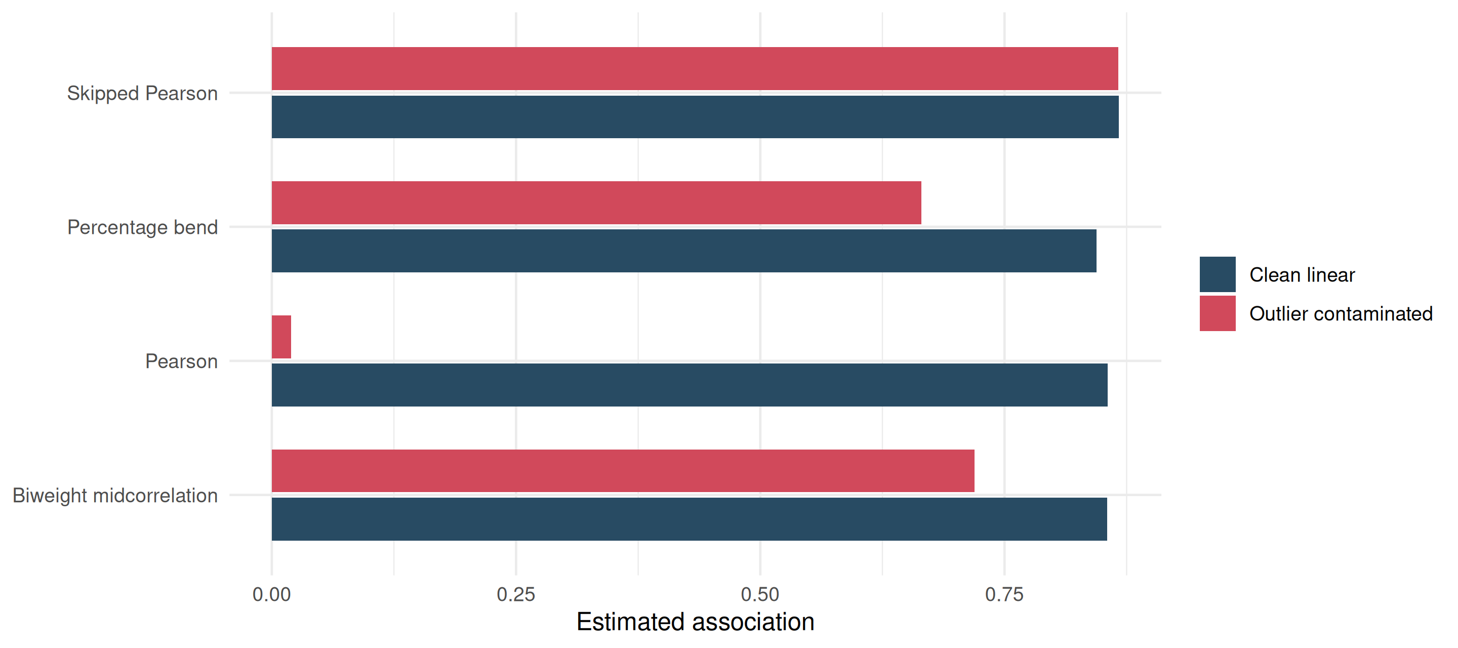
scenario	pearson	bicor	pbcor	skipped
Clean linear	0.856	0.855	0.844	0.867
Outlier contaminated	0.020	0.719	0.665	0.866

Here the robust methods are not automatic replacements for Pearson. They are sensitivity diagnostics. In matrixCorr, the examples are biweight midcorrelation through bicor(), percentage bend correlation through pbcor() and skipped Pearson correlation through skipped_corr(). These methods achieve robustness in different ways. Biweight midcorrelation downweights extreme observations, and percentage bend correlation limits their influence by bending standardised marginal deviations. Skipped correlation identifies multivariate outliers using an explicit outlier detection rule and then computes correlation on the retained observations (Wilcox, 2004; Pernet, Wilcox and Rousselet, 2013). These methods need not estimate the same population functional. The particular detection rule used here is documented under Reproducibility.

If robust correlations disagree substantially with Pearson, the estimated association is sensitive to a small subset of observations. Those points might be measurement errors, data processing problems, or rare but scientifically meaningful cases. This sensitivity analysis does not by itself justify deleting them.

7.2 Range restriction

Contamination concerns particular observations; range restriction concerns sampling only part of the underlying range. Restricting \(X\) can alter correlation even when the regression mechanism remains unchanged (Mendoza and Mumford, 1987). The following comparison retains observations from a narrow central range of \(X\).

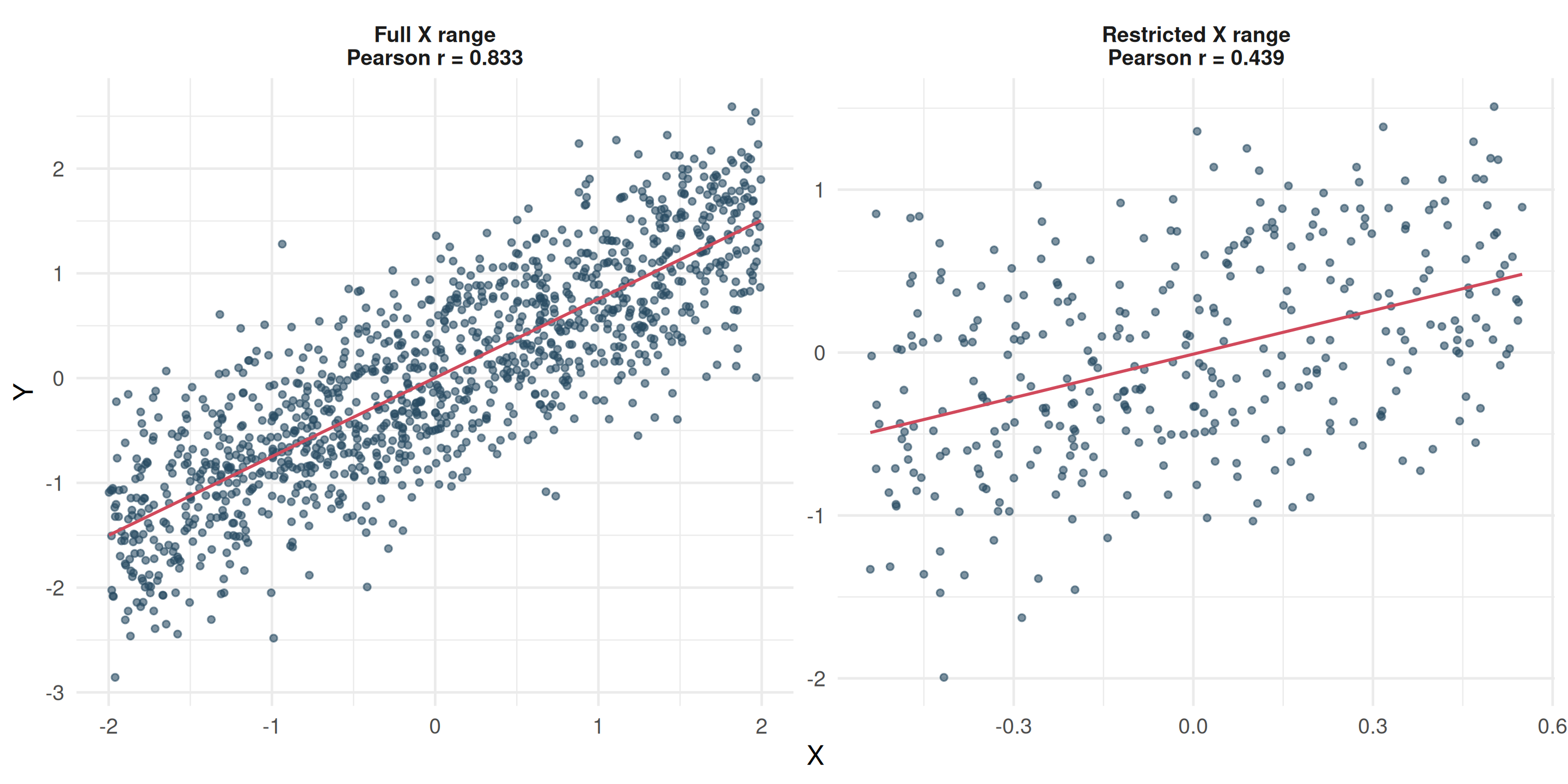
scenario	n	pearson
Full X range	1200	0.833
Restricted X range	349	0.439

8 Marginal and partial correlation

Now create a common cause structure.

\[ Z \sim N(0,1), \qquad X = aZ+\varepsilon_X, \qquad Y=bZ+\varepsilon_Y. \]

The errors are independent centred Gaussian variables, also independent of \(Z\). There is no direct term between \(X\) and \(Y\). Marginally, they move together because both move with \(Z\).

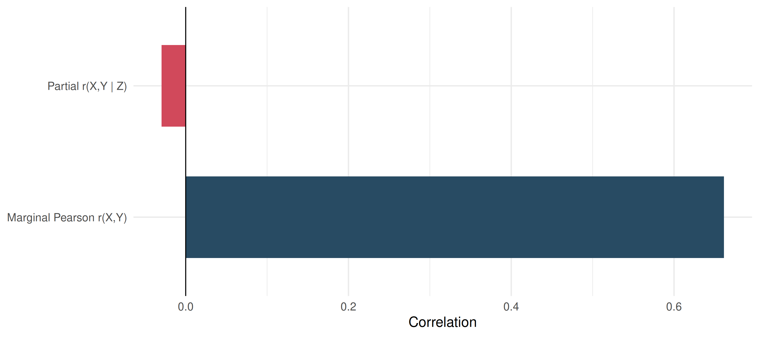
scenario	marginal_pearson	partial_xy_given_z
Common cause only	0.661	-0.03

Conventional partial correlation asks whether residual linear association remains after linearly adjusting for one or more variables. With one adjustment variable \(Z\), the population partial correlation can be written as

\[ \rho_{XY\cdot Z} = \frac{ \rho_{XY}-\rho_{XZ}\rho_{YZ} }{ \sqrt{(1-\rho_{XZ}^{2})(1-\rho_{YZ}^{2})} }. \]

In general,

\[ \rho_{XY\cdot Z}=0 \not\Rightarrow X \perp Y \mid Z. \]

For jointly multivariate Gaussian variables with a nonsingular covariance matrix, zero partial correlation between two variables conditional on the remaining variables is equivalent to conditional independence (Baba, Shibata and Sibuya, 2004).

We know \(Z\) is a common cause here because we constructed the mechanism. Partial correlation does not discover causal structure or establish that an adjustment set is appropriate. That requires assumptions about how the variables were generated.

Conditioning on a collider

Adjustment is not automatically beneficial. A collider has the structure

X -> Z <- Y

Conditioning on a collider can create an association between \(X\) and \(Y\) even when they were marginally independent (Greenland, Pearl and Robins, 1999). The small simulation below uses independent \(X\) and \(Y\), then constructs \(Z\) from both.

scenario	marginal_pearson	partial_xy_given_z
Collider adjustment	0.027	-0.568

“Adjusted” does not automatically mean “closer to the truth”.

9 Final remarks

The measures considered here target different features of the joint distribution. Pearson describes linear association, Spearman and Kendall describe ordering, and distance correlation and HSIC address broader dependence. Chatterjee’s \(\xi\) adds directional dependence, robust estimators examine sensitivity to unusual observations, and partial correlation describes residual linear association after adjustment. They are not competing estimates of a common parameter, and their numerical magnitudes do not share a common interpretation.

Agreement can be reassuring when the measures reflect compatible aspects of a relationship, but disagreement can also be informative. A small Pearson correlation accompanied by general dependence raises a different question from a discrepancy between Pearson and a robust estimator. The useful question is which feature of the joint distribution causes the disagreement, rather than which coefficient is numerically largest.

A coefficient quantifies a selected feature, not the complete joint distribution. Curvature, heteroscedasticity, mixtures, influence and asymmetry can be lost in a single summary. Choosing a measure does not remove the need for scientific assumptions, uncertainty quantification and appropriate modelling.

Describing dependence and making an inferential statement about it are different tasks. A sample coefficient estimates a population quantity, while evidence against independence requires an appropriate sampling or null distribution. Conventional distance correlation and biased empirical HSIC are especially useful reminders of this distinction because their sample values need not be zero under independence (Székely, Rizzo and Bakirov, 2007; Gretton et al., 2007).

The measure should therefore follow the scientific question. If linear association is the target, Pearson may be exactly the right statistic. Add another measure when it addresses a feature left unresolved by that analysis. There is no requirement to calculate every available coefficient.

Before asking “what is the correlation?”, ask “what aspect of this relationship do I want to quantify?”

10 References

Pearson, K. (1896). Mathematical Contributions to the Theory of Evolution. III. Regression, Heredity, and Panmixia. Philosophical Transactions of the Royal Society of London. Series A, 187, 253 to 318.
Spearman, C. (1904). The Proof and Measurement of Association between Two Things. The American Journal of Psychology, 15(1), 72 to 101.
Kendall, M. G. (1938). A New Measure of Rank Correlation. Biometrika, 30(1 to 2), 81 to 93.
Székely, G. J., Rizzo, M. L. and Bakirov, N. K. (2007). Measuring and Testing Dependence by Correlation of Distances. The Annals of Statistics, 35(6), 2769 to 2794.
Gretton, A., Bousquet, O., Smola, A. and Schölkopf, B. (2005). Measuring Statistical Dependence with Hilbert-Schmidt Norms. Algorithmic Learning Theory, Lecture Notes in Computer Science 3734, 63 to 77.
Gretton, A., Fukumizu, K., Teo, C. H., Song, L., Schölkopf, B. and Smola, A. (2007). A Kernel Statistical Test of Independence. Advances in Neural Information Processing Systems.
Dette, H., Siburg, K. F. and Stoimenov, P. A. (2013). A Copula-Based Non-parametric Measure of Regression Dependence. Scandinavian Journal of Statistics, 40(1), 21 to 41.
Chatterjee, S. (2021). A New Coefficient of Correlation. Journal of the American Statistical Association, 116(536), 2009 to 2022.
Shi, H., Drton, M. and Han, F. (2022). On the Power of Chatterjee’s Rank Correlation. Biometrika, 109(2), 317 to 333.
Lin, Z. and Han, F. (2023). On Boosting the Power of Chatterjee’s Rank Correlation. Biometrika, 110(2), 283 to 299.
Lin, Z. and Han, F. (2025). Limit Theorems of Chatterjee’s Rank Correlation. arXiv:2204.08031.
Dette, H. and Kroll, M. (2025). A Simple Bootstrap for Chatterjee’s Rank Correlation. Biometrika, 112(1), asae045.
Dalitz, C., Arning, J. and Goebbels, S. (2024). A Simple Bias Reduction for Chatterjee’s Correlation. Journal of Statistical Theory and Practice, 18, Article 51.
Pernet, C. R., Wilcox, R. and Rousselet, G. A. (2013). Robust Correlation Analyses: False Positive and Power Validation Using a New Open Source Matlab Toolbox. Frontiers in Psychology, 3, Article 606.
Baba, K., Shibata, R. and Sibuya, M. (2004). Partial Correlation and Conditional Correlation as Measures of Conditional Independence. Australian and New Zealand Journal of Statistics, 46(4), 657 to 664.
de Winter, J. C. F., Gosling, S. D. and Potter, J. (2016). Comparing the Pearson and Spearman Correlation Coefficients Across Distributions and Sample Sizes: A Tutorial Using Simulations and Empirical Data. Psychological Methods, 21(3), 273 to 290.
Gretton, A., Herbrich, R., Smola, A., Bousquet, O. and Schölkopf, B. (2005). Kernel Methods for Measuring Independence. Journal of Machine Learning Research, 6, 2075 to 2129.
Sriperumbudur, B. K., Gretton, A., Fukumizu, K., Schölkopf, B. and Lanckriet, G. R. G. (2010). Hilbert Space Embeddings and Metrics on Probability Measures. Journal of Machine Learning Research, 11, 1517 to 1561.
Mendoza, J. L. and Mumford, M. (1987). Corrections for Attenuation and Range Restriction on the Predictor. Journal of Educational Statistics, 12(3), 282 to 293.
Wilcox, R. R. (2004). Inferences Based on a Skipped Correlation Coefficient. Journal of Applied Statistics, 31(2), 131 to 143.
Greenland, S., Pearl, J. and Robins, J. M. (1999). Causal Diagrams for Epidemiologic Research. Epidemiology, 10(1), 37 to 48.

11 Reproducibility

The package behaviour was verified against the current matrixCorr GitHub implementation, version 0.12.3. The figures and tables in this article use that implementation. The following are software conventions, separate from the population results cited above.

matrixCorr::dcor() returns the conventional nonnegative sample distance correlation \(R_n\) from doubly centred distance matrices. dcor(squared = TRUE) returns \(R_n^2\). The separate bcdcor() function returns the signed, U centred bias corrected squared distance correlation statistic, which can be negative in finite samples.

matrixCorr::dcor(p_value = TRUE) reports conventional distance correlation in the displayed matrix, while the attached independence test metadata use the signed bias corrected statistic returned by bcdcor(). The attached t test is not computed directly from the displayed \(R_n\). matrixCorr::hsic(p_value = TRUE) can attach permutation p values; this article uses its normalised biased estimator with Gaussian kernels and median bandwidths.

The default xi_corr() returns the original finite sample statistic. bias_correction = "upper_bound" divides it by its finite sample upper bound, leaving the population target unchanged. For skipped Pearson correlation, this implementation uses a projection based bivariate outlier rule for each variable pair, then computes Pearson correlation on the retained observations.

The main text hides R chunks so the statistical narrative stays readable. Open the panel below to inspect the reusable simulation and plotting code.

Reusable R code

# Reusable simulations and plotting helpers for the "Beyond Pearson" post.

BEYOND_PEARSON <- list(
  seed = 20260927L,
  n = 500L,
  rho_linear = 0.70,
  monotonic_a = 0.85,
  monotonic_noise = 0.45,
  quadratic_noise = 0.35,
  periodic_noise = 0.35,
  outlier_n = 400L,
  outlier_fraction = 0.04,
  outlier_noise = 0.45,
  opening_outlier_scale = 0.77,
  range_n = 1200L,
  range_restriction = 0.55,
  confound_a = 0.85,
  confound_b = 0.80,
  confound_noise = 0.55,
  confound_direct = 0.25,
  collider_a = 0.80,
  collider_b = 0.80,
  collider_noise = 0.65
)

required_packages <- function() {
  required <- c("matrixCorr", "ggplot2", "knitr")
  missing <- required[!vapply(required, requireNamespace, logical(1), quietly = TRUE)]
  if (length(missing) > 0L) {
    stop("Install required packages: ", paste(missing, collapse = ", "), call. = FALSE)
  }
  if (!"bcdcor" %in% getNamespaceExports("matrixCorr") ||
      !"squared" %in% names(formals(matrixCorr::dcor))) {
    stop(paste(
      "Install the current GitHub matrixCorr implementation with conventional dcor() and bcdcor().",
      "Follow the project .Rlib installation instructions in the post README and restart R if matrixCorr is already loaded."
    ),
         call. = FALSE)
  }
  invisible(TRUE)
}

simulate_relationship <- function(type,
                                  n = BEYOND_PEARSON$n,
                                  seed = BEYOND_PEARSON$seed,
                                  noise = NULL,
                                  rho = BEYOND_PEARSON$rho_linear) {
  type <- match.arg(
    type,
    c(
      "independent", "linear", "monotonic", "quadratic", "periodic",
      "outlier_clean", "outlier_contaminated",
      "confounded", "confounded_direct", "collider",
      "range_full", "range_restricted",
      "opening_linear", "opening_curved", "opening_outliers",
      "opening_heteroscedastic", "opening_mixture"
    )
  )
  set.seed(seed)

  if (type == "independent") {
    x <- rnorm(n)
    y <- rnorm(n)
    return(data.frame(scenario = "Independent Gaussian", x = x, y = y))
  }

  if (type == "linear") {
    x <- rnorm(n)
    eps <- rnorm(n)
    y <- rho * x + sqrt(1 - rho^2) * eps
    return(data.frame(scenario = "Linear Gaussian", x = x, y = y))
  }

  if (type == "monotonic") {
    sigma <- noise %||% BEYOND_PEARSON$monotonic_noise
    x <- rnorm(n)
    y <- exp(BEYOND_PEARSON$monotonic_a * x) + rnorm(n, sd = sigma)
    return(data.frame(scenario = "Monotonic nonlinear", x = x, y = y))
  }

  if (type == "quadratic") {
    sigma <- noise %||% BEYOND_PEARSON$quadratic_noise
    x <- rnorm(n)
    y <- x^2 + rnorm(n, sd = sigma)
    return(data.frame(scenario = "Quadratic", x = x, y = y))
  }

  if (type == "periodic") {
    sigma <- noise %||% BEYOND_PEARSON$periodic_noise
    x <- runif(n, -pi, pi)
    y <- sin(2 * x) + rnorm(n, sd = sigma)
    return(data.frame(scenario = "Periodic", x = x, y = y))
  }

  if (type %in% c("outlier_clean", "outlier_contaminated")) {
    n <- BEYOND_PEARSON$outlier_n
    x <- rnorm(n)
    y <- 0.8 * x + rnorm(n, sd = BEYOND_PEARSON$outlier_noise)
    contaminated <- rep(FALSE, n)
    if (type == "outlier_contaminated") {
      m <- max(1L, round(BEYOND_PEARSON$outlier_fraction * n))
      idx <- sample(seq_len(n), m)
      contaminated[idx] <- TRUE
      x[idx] <- x[idx] + runif(m, 3.5, 5.0)
      y[idx] <- y[idx] - runif(m, 3.5, 5.0)
    }
    label <- if (type == "outlier_clean") "Clean linear" else "Outlier contaminated"
    return(data.frame(scenario = label, x = x, y = y, contaminated = contaminated))
  }

  if (type %in% c("confounded", "confounded_direct")) {
    z <- rnorm(n)
    x <- BEYOND_PEARSON$confound_a * z + rnorm(n, sd = BEYOND_PEARSON$confound_noise)
    direct <- if (type == "confounded_direct") BEYOND_PEARSON$confound_direct else 0
    y <- BEYOND_PEARSON$confound_b * z + direct * x + rnorm(n, sd = BEYOND_PEARSON$confound_noise)
    label <- if (type == "confounded") "Common cause only" else "Common cause plus direct association"
    return(data.frame(scenario = label, x = x, y = y, z = z))
  }

  if (type == "collider") {
    x <- rnorm(n)
    y <- rnorm(n)
    z <- BEYOND_PEARSON$collider_a * x + BEYOND_PEARSON$collider_b * y +
      rnorm(n, sd = BEYOND_PEARSON$collider_noise)
    return(data.frame(scenario = "Collider adjustment", x = x, y = y, z = z))
  }

  if (type %in% c("range_full", "range_restricted")) {
    n_full <- max(n, BEYOND_PEARSON$range_n)
    x_full <- runif(n_full, -2, 2)
    y_full <- 0.75 * x_full + rnorm(n_full, sd = 0.55)
    if (type == "range_restricted") {
      keep <- abs(x_full) <= BEYOND_PEARSON$range_restriction
      x_full <- x_full[keep]
      y_full <- y_full[keep]
      label <- "Restricted X range"
    } else {
      label <- "Full X range"
    }
    return(data.frame(scenario = label, x = x_full, y = y_full))
  }

  if (type == "opening_linear") {
    x <- rnorm(n)
    y <- 0.60 * x + sqrt(1 - 0.60^2) * rnorm(n)
    return(data.frame(scenario = "Gaussian linear", x = x, y = y))
  }

  if (type == "opening_curved") {
    x <- rnorm(n)
    y <- exp(0.65 * x) + rnorm(n, sd = 0.85)
    return(data.frame(scenario = "Curved monotonic", x = x, y = y))
  }

  if (type == "opening_outliers") {
    dat <- simulate_relationship("outlier_clean", seed = seed)
    # Spread isolated points across both sides of the cloud, with varied
    # offsets and equal numbers above and below the main trend.
    # The fixed scale gives r about 0.78 for the opening figure's seed.
    m <- 2L * max(1L, round(BEYOND_PEARSON$outlier_fraction * nrow(dat) / 2L))
    idx <- sample(seq_len(nrow(dat)), m)
    dat$x[idx] <- seq(-6, 6, length.out = m) + runif(m, -0.25, 0.25)
    direction <- sample(rep(c(-1, 1), each = m / 2L))
    magnitude <- runif(m, 2, 5.5)
    dat$y[idx] <- 0.8 * dat$x[idx] +
      direction * magnitude * BEYOND_PEARSON$opening_outlier_scale
    dat$scenario <- "Influential observations"
    return(dat[, c("scenario", "x", "y")])
  }

  if (type == "opening_heteroscedastic") {
    x <- rnorm(n)
    y <- 0.62 * x + rnorm(n, sd = 0.25 + 0.55 * abs(x))
    return(data.frame(scenario = "Heteroscedastic", x = x, y = y))
  }

  x <- c(rnorm(n / 2L, -1.2, 0.55), rnorm(n - n / 2L, 1.2, 0.55))
  y <- c(rnorm(n / 2L, -0.55, 0.45), rnorm(n - n / 2L, 0.95, 0.45))
  data.frame(scenario = "Two clusters", x = x, y = y)
}

`%||%` <- function(x, y) {
  if (is.null(x)) y else x
}

pair_value <- function(object, x_name = "x", y_name = "y") {
  unname(as.matrix(object)[x_name, y_name])
}

safe_pair_value <- function(expr) {
  tryCatch(expr, error = function(e) NA_real_)
}

summarise_dependence <- function(x, y,
                                 include_robust = TRUE,
                                 hsic_normalise = TRUE,
                                 xi_bias_correction = "none",
                                 xi_tie_method = "random",
                                 xi_seed = BEYOND_PEARSON$seed + 9000L) {
  required_packages()
  xy <- cbind(x = x, y = y)
  out <- data.frame(
    n = length(x),
    pearson = safe_pair_value(pair_value(matrixCorr::pearson_corr(xy))),
    spearman = safe_pair_value(pair_value(matrixCorr::spearman_rho(xy))),
    kendall = safe_pair_value(pair_value(matrixCorr::kendall_tau(xy))),
    dcor = safe_pair_value(pair_value(matrixCorr::dcor(xy, squared = FALSE))),
    hsic = safe_pair_value(pair_value(matrixCorr::hsic(
      xy,
      kernel = "gaussian",
      bandwidth = "median",
      normalise = hsic_normalise,
      estimator = "biased"
    ))),
    xi_y_given_x = safe_pair_value(matrixCorr::xi_corr(
      x,
      y,
      tie_method = xi_tie_method,
      seed = xi_seed,
      bias_correction = xi_bias_correction
    )),
    xi_x_given_y = safe_pair_value(matrixCorr::xi_corr(
      y,
      x,
      tie_method = xi_tie_method,
      seed = xi_seed,
      bias_correction = xi_bias_correction
    ))
  )

  if (include_robust) {
    out$bicor <- safe_pair_value(pair_value(matrixCorr::bicor(xy)))
    out$pbcor <- safe_pair_value(pair_value(matrixCorr::pbcor(xy)))
    out$skipped <- safe_pair_value(pair_value(matrixCorr::skipped_corr(xy)))
  }

  out
}

main_scenarios <- function() {
  types <- c("linear", "monotonic", "quadratic", "periodic")
  seeds <- BEYOND_PEARSON$seed + seq_along(types) - 1L
  stats::setNames(
    Map(simulate_relationship, types, seed = seeds),
    c("Linear", "Monotonic nonlinear", "Quadratic", "Periodic")
  )
}

opening_scenarios <- function() {
  types <- c(
    "opening_linear", "opening_curved", "opening_outliers",
    "opening_heteroscedastic", "opening_mixture"
  )
  seeds <- BEYOND_PEARSON$seed + 100L + seq_along(types)
  stats::setNames(Map(simulate_relationship, types, seed = seeds), types)
}

summary_table <- function(scenarios) {
  rows <- lapply(scenarios, function(dat) {
    cbind(
      scenario = unique(dat$scenario)[1L],
      summarise_dependence(dat$x, dat$y)
    )
  })
  do.call(rbind, rows)
}

partial_summary <- function(dat) {
  xyz <- cbind(x = dat$x, y = dat$y, z = dat$z)
  data.frame(
    scenario = unique(dat$scenario)[1L],
    marginal_pearson = pair_value(matrixCorr::pearson_corr(xyz[, c("x", "y")])),
    partial_xy_given_z = pair_value(matrixCorr::pcorr(xyz, method = "sample"), "x", "y")
  )
}

range_summary <- function(full, restricted) {
  data.frame(
    scenario = c(unique(full$scenario)[1L], unique(restricted$scenario)[1L]),
    n = c(nrow(full), nrow(restricted)),
    pearson = c(
      pair_value(matrixCorr::pearson_corr(cbind(x = full$x, y = full$y))),
      pair_value(matrixCorr::pearson_corr(cbind(x = restricted$x, y = restricted$y)))
    )
  )
}

format_stat <- function(x) {
  ifelse(is.na(x), "NA", sprintf("%.3f", x))
}

round_numeric_df <- function(x, digits = 3L) {
  numeric_cols <- vapply(x, is.numeric, logical(1))
  x[numeric_cols] <- lapply(x[numeric_cols], round, digits = digits)
  x
}

plot_relationship <- function(dat, title = unique(dat$scenario)[1L]) {
  required_packages()
  stats <- summarise_dependence(dat$x, dat$y, include_robust = FALSE)
  subtitle <- paste(
    "Pearson r =", format_stat(stats$pearson),
    "| Spearman rho =", format_stat(stats$spearman),
    "| Kendall tau =", format_stat(stats$kendall),
    "| dCor =", format_stat(stats$dcor)
  )
  ggplot2::ggplot(dat, ggplot2::aes(x, y)) +
    ggplot2::geom_point(alpha = 0.68, size = 1.4, color = "#2f4858") +
    ggplot2::geom_smooth(method = "lm", se = FALSE, linewidth = 0.75, color = "#d1495b") +
    ggplot2::labs(title = title, subtitle = subtitle, x = "X", y = "Y") +
    ggplot2::theme_minimal(base_size = 12)
}

plot_shape_panels <- function(scenarios) {
  required_packages()
  dat <- do.call(rbind, scenarios)
  dat$scenario <- factor(
    dat$scenario,
    levels = c("Linear Gaussian", "Monotonic nonlinear", "Quadratic", "Periodic")
  )
  stats <- summary_table(scenarios)
  labels <- setNames(
    paste0(stats$scenario, "\nPearson r = ", format_stat(stats$pearson),
           ", dCor = ", format_stat(stats$dcor)),
    stats$scenario
  )
  ggplot2::ggplot(dat, ggplot2::aes(x, y)) +
    ggplot2::geom_point(alpha = 0.62, size = 1.15, color = "#284b63") +
    ggplot2::geom_smooth(method = "lm", se = FALSE, linewidth = 0.55, color = "#d1495b") +
    ggplot2::facet_wrap(
      ggplot2::vars(scenario),
      scales = "free",
      labeller = ggplot2::as_labeller(labels)
    ) +
    ggplot2::labs(x = "X", y = "Y") +
    ggplot2::theme_minimal(base_size = 11) +
    ggplot2::theme(strip.text = ggplot2::element_text(face = "bold"))
}

long_measure_table <- function(tab,
                               measures = c(
                                 "pearson", "spearman", "kendall", "dcor",
                                 "hsic", "xi_y_given_x", "xi_x_given_y"
                               )) {
  long <- do.call(rbind, lapply(measures, function(measure) {
    data.frame(
      scenario = tab$scenario,
      measure = measure,
      value = as.numeric(tab[[measure]])
    )
  }))
  labels <- c(
    pearson = "Pearson",
    spearman = "Spearman",
    kendall = "Kendall",
    dcor = "Distance correlation",
    hsic = "Normalised HSIC",
    xi_y_given_x = "xi(X, Y) for Y given X",
    xi_x_given_y = "xi(Y, X) for X given Y",
    bicor = "Biweight midcorrelation",
    pbcor = "Percentage bend",
    skipped = "Skipped Pearson"
  )
  long$measure_label <- unname(labels[long$measure])
  long
}

plot_measure_small_multiples <- function(tab) {
  required_packages()
  long <- long_measure_table(tab)
  ggplot2::ggplot(long, ggplot2::aes(scenario, value, fill = scenario)) +
    ggplot2::geom_col(width = 0.72, show.legend = FALSE) +
    ggplot2::facet_wrap(ggplot2::vars(measure_label), scales = "free_y") +
    ggplot2::coord_flip() +
    ggplot2::labs(
      x = NULL,
      y = "Estimated value",
      caption = "Compare patterns within each measure."
    ) +
    ggplot2::scale_fill_manual(values = c("#2f4858", "#688e26", "#d1495b", "#5b5f97", "#7f7f7f")) +
    ggplot2::theme_minimal(base_size = 11)
}

plot_pearson_dcor <- function(tab) {
  required_packages()
  long <- long_measure_table(tab, measures = c("pearson", "dcor"))
  ggplot2::ggplot(long, ggplot2::aes(scenario, value, fill = measure_label)) +
    ggplot2::geom_col(position = ggplot2::position_dodge(width = 0.72), width = 0.64) +
    ggplot2::coord_flip() +
    ggplot2::labs(
      x = NULL,
      y = "Estimated value",
      fill = NULL,
      caption = "Compare the quadratic scenario with the other simulated relationships."
    ) +
    ggplot2::scale_fill_manual(values = c("Distance correlation" = "#688e26", "Pearson" = "#d1495b")) +
    ggplot2::theme_minimal(base_size = 12)
}

plot_xi_direction <- function(tab) {
  required_packages()
  long <- long_measure_table(tab, measures = c("xi_y_given_x", "xi_x_given_y"))
  ggplot2::ggplot(long, ggplot2::aes(scenario, value, fill = measure_label)) +
    ggplot2::geom_col(position = ggplot2::position_dodge(width = 0.72), width = 0.64) +
    ggplot2::coord_flip() +
    ggplot2::labs(
      x = NULL,
      y = "Chatterjee xi",
      fill = NULL,
      caption = "Compare the two argument orders within each scenario."
    ) +
    ggplot2::scale_fill_manual(values = c(
      "xi(X, Y) for Y given X" = "#284b63",
      "xi(Y, X) for X given Y" = "#f4a261"
    )) +
    ggplot2::theme_minimal(base_size = 12)
}

plot_robustness <- function(clean, contaminated) {
  required_packages()
  dat <- rbind(clean, contaminated)
  dat$scenario <- factor(dat$scenario, levels = c("Clean linear", "Outlier contaminated"))
  robust <- rbind(
    cbind(scenario = "Clean linear", summarise_dependence(clean$x, clean$y)),
    cbind(scenario = "Outlier contaminated", summarise_dependence(contaminated$x, contaminated$y))
  )
  long <- long_measure_table(
    robust,
    measures = c("pearson", "bicor", "pbcor", "skipped")
  )
  scatter <- ggplot2::ggplot(dat, ggplot2::aes(x, y)) +
    ggplot2::geom_point(
      ggplot2::aes(color = contaminated),
      alpha = 0.68,
      size = 1.2,
      show.legend = FALSE
    ) +
    ggplot2::geom_smooth(method = "lm", se = FALSE, linewidth = 0.6, color = "#d1495b") +
    ggplot2::facet_wrap(ggplot2::vars(scenario), scales = "free") +
    ggplot2::scale_color_manual(values = c("FALSE" = "#284b63", "TRUE" = "#f4a261")) +
    ggplot2::labs(x = "X", y = "Y") +
    ggplot2::theme_minimal(base_size = 11)
  bars <- ggplot2::ggplot(long, ggplot2::aes(measure_label, value, fill = scenario)) +
    ggplot2::geom_col(position = ggplot2::position_dodge(width = 0.72), width = 0.64) +
    ggplot2::coord_flip() +
    ggplot2::labs(x = NULL, y = "Estimated association", fill = NULL) +
    ggplot2::scale_fill_manual(values = c("Clean linear" = "#284b63", "Outlier contaminated" = "#d1495b")) +
    ggplot2::theme_minimal(base_size = 11)
  list(scatter = scatter, bars = bars, table = robust)
}

plot_partial <- function(dat) {
  required_packages()
  ps <- partial_summary(dat)
  long <- data.frame(
    measure = c("Marginal Pearson r(X,Y)", "Partial r(X,Y | Z)"),
    value = c(ps$marginal_pearson, ps$partial_xy_given_z)
  )
  ggplot2::ggplot(long, ggplot2::aes(measure, value, fill = measure)) +
    ggplot2::geom_col(width = 0.62, show.legend = FALSE) +
    ggplot2::coord_flip() +
    ggplot2::geom_hline(yintercept = 0, linewidth = 0.4) +
    ggplot2::labs(x = NULL, y = "Correlation") +
    ggplot2::scale_fill_manual(values = c("#284b63", "#d1495b")) +
    ggplot2::theme_minimal(base_size = 12)
}

# Exact population conversions under a bivariate normal model.
gaussian_correlations <- function(value,
                                  from = c("pearson", "spearman", "kendall")) {
  from <- match.arg(from)
  if (!is.numeric(value) || length(value) == 0L ||
      any(!is.finite(value)) || any(abs(value) > 1)) {
    stop("value must contain finite numeric correlations between -1 and 1.",
         call. = FALSE)
  }
  rho <- switch(from,
    pearson = value,
    spearman = 2 * sin(pi * value / 6),
    kendall = sin(pi * value / 2)
  )
  # Preserve exact endpoints despite floating-point sine evaluation.
  rho[abs(value) == 1] <- sign(value[abs(value) == 1])
  # Gaussian population dCor squared, with rationalised square-root terms
  # to avoid cancellation near independence.
  dcor_squared <- (
    rho * (asin(rho) - asin(rho / 2)) +
      rho^2 * (1 / (2 + sqrt(4 - rho^2)) -
                 1 / (1 + sqrt(1 - rho^2)))
  ) / (1 + pi / 3 - sqrt(3))
  data.frame(
    pearson = rho,
    spearman = 6 / pi * asin(rho / 2),
    kendall = 2 / pi * asin(rho),
    dcor = sqrt(pmax(0, pmin(1, dcor_squared)))
  )
}


gaussian_special_case <- function(rhos = seq(-1, 1, by = 0.1),
                                  n = 2500L,
                                  seed = BEYOND_PEARSON$seed + 2000L) {
  rows <- lapply(seq_along(rhos), function(i) {
    rho <- rhos[i]
    dat <- simulate_relationship("linear", n = n, seed = seed + i, rho = rho)
    cbind(rho = rho, summarise_dependence(dat$x, dat$y, include_robust = FALSE))
  })
  out <- do.call(rbind, rows)
  out$scenario <- paste0("rho = ", out$rho)
  out
}

plot_gaussian_special_case <- function(tab) {
  required_packages()
  tab$scenario <- sprintf("rho = %.1f", tab$rho)
  measures <- c("pearson", "spearman", "kendall", "dcor")
  long <- long_measure_table(tab, measures = measures)
  long$rho <- rep(tab$rho, length(measures))
  # Evaluate the population formulas on a dense grid for smooth reference curves.
  theory_rhos <- seq(-1, 1, length.out = 501L)
  theory_tab <- gaussian_correlations(theory_rhos)
  theory_tab$scenario <- as.character(theory_rhos)
  theory <- long_measure_table(theory_tab, measures = measures)
  theory$rho <- rep(theory_rhos, length(measures))
  ggplot2::ggplot(long, ggplot2::aes(rho, value, color = measure_label)) +
    ggplot2::geom_line(
      data = theory,
      ggplot2::aes(rho, value, color = measure_label),
      linewidth = 0.8,
      linetype = "22"
    ) +
    ggplot2::geom_line(linewidth = 0.8) +
    ggplot2::geom_point(size = 1.7) +
    ggplot2::scale_color_manual(values = c(
      "Pearson" = "#00BA38", "Spearman" = "#619CFF",
      "Kendall" = "#F8766D", "Distance correlation" = "#8844AA"
    )) +
    ggplot2::scale_x_continuous(breaks = seq(-1, 1, by = 0.5)) +
    ggplot2::scale_y_continuous(breaks = seq(-1, 1, by = 0.5)) +
    ggplot2::coord_cartesian(xlim = c(-1, 1), ylim = c(-1, 1)) +
    ggplot2::labs(
      x = "Population Pearson rho used to generate bivariate normal data",
      y = "Correlation coefficient",
      color = NULL,
      caption = "Solid lines are simulated estimates. Dashed lines are the Gaussian reference formulas."
    ) +
    ggplot2::theme_minimal(base_size = 12)
}

plot_opening_same_pearson <- function(scenarios) {
  required_packages()
  dat <- do.call(rbind, scenarios)
  stats <- summary_table(scenarios)
  labels <- setNames(
    paste0(stats$scenario, "\nPearson r = ", format_stat(stats$pearson)),
    stats$scenario
  )
  ggplot2::ggplot(dat, ggplot2::aes(x, y)) +
    ggplot2::geom_point(alpha = 0.62, size = 1.1, color = "#2f4858") +
    ggplot2::geom_smooth(method = "lm", se = FALSE, linewidth = 0.55, color = "#d1495b") +
    ggplot2::facet_wrap(
      ggplot2::vars(scenario),
      scales = "free",
      labeller = ggplot2::as_labeller(labels)
    ) +
    ggplot2::labs(x = "X", y = "Y") +
    ggplot2::theme_minimal(base_size = 11) +
    ggplot2::theme(strip.text = ggplot2::element_text(face = "bold"))
}

monte_carlo_stability <- function(types = c("independent", "linear", "quadratic", "periodic"),
                                  reps = 200L,
                                  n = 300L,
                                  seed = BEYOND_PEARSON$seed + 5000L) {
  rows <- list()
  k <- 1L
  for (type in types) {
    for (r in seq_len(reps)) {
      dat <- simulate_relationship(type, n = n, seed = seed + 1000L * match(type, types) + r)
      stats <- summarise_dependence(dat$x, dat$y, include_robust = FALSE)
      rows[[k]] <- cbind(type = type, replicate = r, stats)
      k <- k + 1L
    }
  }
  do.call(rbind, rows)
}

monte_carlo_summary <- function(mc,
                                measures = c("pearson", "spearman", "dcor", "xi_y_given_x")) {
  out <- do.call(rbind, lapply(split(mc, mc$type), function(dat) {
    do.call(rbind, lapply(measures, function(measure) {
      values <- as.numeric(dat[[measure]])
      data.frame(
        scenario = unique(dat$type),
        measure = measure,
        mean = mean(values, na.rm = TRUE),
        sd = stats::sd(values, na.rm = TRUE),
        q025 = unname(stats::quantile(values, 0.025, na.rm = TRUE)),
        median = stats::median(values, na.rm = TRUE),
        q975 = unname(stats::quantile(values, 0.975, na.rm = TRUE))
      )
    }))
  }))
  rownames(out) <- NULL
  out
}

validate_xi_direction <- function(n = 500L) {
  set.seed(BEYOND_PEARSON$seed + 7000L)
  x <- stats::runif(n, -1, 1)
  y <- x^2
  xi_y_given_x <- matrixCorr::xi_corr(x, y)
  xi_x_given_y <- matrixCorr::xi_corr(y, x)
  data.frame(
    xi_y_given_x = xi_y_given_x,
    xi_x_given_y = xi_x_given_y,
    direction_confirmed = xi_y_given_x > xi_x_given_y
  )
}

plot_range_restriction <- function(full, restricted) {
  required_packages()
  dat <- rbind(full, restricted)
  dat$scenario <- factor(dat$scenario, levels = c("Full X range", "Restricted X range"))
  stats <- range_summary(full, restricted)
  labels <- setNames(
    paste0(stats$scenario, "\nPearson r = ", format_stat(stats$pearson)),
    stats$scenario
  )
  ggplot2::ggplot(dat, ggplot2::aes(x, y)) +
    ggplot2::geom_point(alpha = 0.60, size = 1.05, color = "#284b63") +
    ggplot2::geom_smooth(method = "lm", se = FALSE, linewidth = 0.6, color = "#d1495b") +
    ggplot2::facet_wrap(
      ggplot2::vars(scenario),
      scales = "free",
      labeller = ggplot2::as_labeller(labels)
    ) +
    ggplot2::labs(x = "X", y = "Y") +
    ggplot2::theme_minimal(base_size = 11) +
    ggplot2::theme(strip.text = ggplot2::element_text(face = "bold"))
}

plot_workflow <- function() {
  required_packages()
  nodes <- data.frame(
    label = c(
      "Scientific question",
      "Plot X against Y",
      "Approximately linear?\nPearson",
      "Ordered but curved?\nSpearman or Kendall",
      "Nonmonotonic dependence?\ndCor or HSIC",
      "Direction relevant?\nChatterjee xi",
      "Influential observations?\nRobust sensitivity",
      "Adjustment needed?\nPartial correlation or model"
    ),
    x = c(0, 0, -2.7, -1.35, 0, 1.35, 2.7, 0),
    y = c(3, 2, 0.75, 0.75, 0.75, 0.75, 0.75, -0.65)
  )
  edges <- data.frame(
    x = c(0, 0, 0, 0, 0, 0, 0),
    y = c(2.8, 1.8, 1.8, 1.8, 1.8, 1.8, 0.45),
    xend = c(0, -2.7, -1.35, 0, 1.35, 2.7, 0),
    yend = c(2.25, 1.05, 1.05, 1.05, 1.05, 1.05, -0.35)
  )
  ggplot2::ggplot() +
    ggplot2::geom_segment(
      data = edges,
      ggplot2::aes(x = x, y = y, xend = xend, yend = yend),
      linewidth = 0.45,
      color = "#6b7280",
      arrow = ggplot2::arrow(length = grid::unit(0.12, "inches"))
    ) +
    ggplot2::geom_label(
      data = nodes,
      ggplot2::aes(x = x, y = y, label = label),
      label.size = 0.25,
      size = 3.2,
      fill = "#f8fafc",
      color = "#111827"
    ) +
    ggplot2::coord_cartesian(xlim = c(-3.6, 3.6), ylim = c(-1.2, 3.4), expand = FALSE) +
    ggplot2::theme_void(base_size = 12)
}

## R version 4.6.1 (2026-06-24)
## Platform: x86_64-pc-linux-gnu
## Running under: Ubuntu 24.04.5 LTS
## 
## Matrix products: default
## BLAS:   /usr/lib/x86_64-linux-gnu/openblas-pthread/libblas.so.3 
## LAPACK: /usr/lib/x86_64-linux-gnu/openblas-pthread/libopenblasp-r0.3.26.so;  LAPACK version 3.12.0
## 
## locale:
##  [1] LC_CTYPE=en_GB.UTF-8       LC_NUMERIC=C              
##  [3] LC_TIME=en_GB.UTF-8        LC_COLLATE=en_GB.UTF-8    
##  [5] LC_MONETARY=en_GB.UTF-8    LC_MESSAGES=en_GB.UTF-8   
##  [7] LC_PAPER=en_GB.UTF-8       LC_NAME=C                 
##  [9] LC_ADDRESS=C               LC_TELEPHONE=C            
## [11] LC_MEASUREMENT=en_GB.UTF-8 LC_IDENTIFICATION=C       
## 
## time zone: Europe/London
## tzcode source: system (glibc)
## 
## attached base packages:
## [1] stats     graphics  grDevices utils     datasets  methods   base     
## 
## loaded via a namespace (and not attached):
##  [1] Matrix_1.7-5       gtable_0.3.6       jsonlite_2.0.0     dplyr_1.2.1       
##  [5] compiler_4.6.1     tidyselect_1.2.1   Rcpp_1.1.1-1.1     dichromat_2.0-0.1 
##  [9] jquerylib_0.1.4    splines_4.6.1      scales_1.4.0       yaml_2.3.12       
## [13] fastmap_1.2.0      lattice_0.23-1     ggplot2_4.0.3      R6_2.6.1          
## [17] labeling_0.4.3     generics_0.1.4     matrixCorr_0.12.3  knitr_1.51        
## [21] tibble_3.3.1       bookdown_0.46      bslib_0.11.0       pillar_1.11.1     
## [25] RColorBrewer_1.1-3 rlang_1.2.0        cachem_1.1.0       xfun_0.58         
## [29] sass_0.4.10        S7_0.2.2           otel_0.2.0         cli_3.6.6         
## [33] mgcv_1.9-4         withr_3.0.2        magrittr_2.0.5     digest_0.6.39     
## [37] grid_4.6.1         rstudioapi_0.18.0  nlme_3.1-169       lifecycle_1.0.5   
## [41] vctrs_0.7.3        evaluate_1.0.5     glue_1.8.1         farver_2.1.2      
## [45] blogdown_1.24      rmarkdown_2.31     tools_4.6.1        pkgconfig_2.0.3   
## [49] htmltools_0.5.9

Beyond Pearson. What else can we learn about the relationship between two variables?