Benchmarking Kendall's Tau in R and Rcpp
1 Overview
This post shows how to go from a quick R prototype to a compiled implementation with Rcpp, using Kendall’s rank correlation as a worked example. We implement fast, \(O(n\log n)\), estimators for both \(\tau_a\) (via a merge-sort inversion count) and \(\tau_b\) (via a Binary Indexed Tree/Fenwick tree with explicit tie counts), then check their accuracy and speed against stats::cor(..., method = "kendall").
2 Setup
knitr::opts_chunk$set(cache = TRUE, autodep = TRUE)

library(Rcpp)
library(microbenchmark)
library(dplyr)
library(ggplot2)
library(knitr)
library(matrixCorr)
library(pcaPP)
set.seed(1)
3 Kendall’s tau definitions
Before diving into code and C++ implementations, let’s understand what we’re computing. Kendall’s tau is a rank-based measure of monotonic association. It contrasts how often pairs of observations agree in order (concordant) versus disagree (discordant). Ties can be handled either by leaving the denominator as the total number of pairs defined here as \(\tau_a\) or by rescaling to discount tied pairs defined here as \(\tau_b\).
Let \(\{(x_i,y_i)\}_{i=1}^n\) be paired observations, and consider all unordered index pairs \((i,j)\) with \(i<j\). For each pair define
\[ s_{ij} \,=\, \operatorname{sgn}(x_i-x_j)\,\operatorname{sgn}(y_i-y_j), \]
with the convention \(\operatorname{sgn}(0)=0\). Thus, \(s_{ij}=+1\) for concordant, \(-1\) for discordant, and \(0\) if the pair is tied in \(x\) or in \(y\) (or both).
Classify pairs:
- Concordant if \((x_i-x_j)(y_i-y_j)>0\).
- Discordant if \((x_i-x_j)(y_i-y_j)<0\).
- Tie in \(x\) if \(x_i=x_j\) (regardless of \(y\)).
- Tie in \(y\) if \(y_i=y_j\) (regardless of \(x\)).
Define the counts
\[ C = \sum_{1\le i<j\le n} \mathbf{1}\!\big((x_i-x_j)(y_i-y_j)>0\big),\quad D = \sum_{1\le i<j\le n} \mathbf{1}\!\big((x_i-x_j)(y_i-y_j)<0\big), \]
and let \(n_0=\binom{n}{2}\) be the total number of pairs.
If the \(x\)-values contain tie groups of sizes \(\{t_{x,g}\}\) and the \(y\)-values tie groups \(\{t_{y,h}\}\), the numbers of tied pairs (counting all ties, including pairs tied on both variables) are
\[ T_x = \sum_g \binom{t_{x,g}}{2}, \qquad T_y = \sum_h \binom{t_{y,h}}{2}. \]
Let \(T_{xy}\) be the number of pairs tied on both variables. Then the calculating identities
\[ n_0 = C + D + T_x + T_y - T_{xy}, \qquad \sum_{i<j} s_{ij} = C - D \]
hold.
3.1 Kendall’s \(\tau_a\) (no tie correction)
\[ \tau_a \,=\, \frac{C - D}{n_0} \,=\, \frac{1}{n_0}\sum_{i<j} s_{ij}. \]
This coefficient lies in \([-1,1]\). It is appropriate when ties are absent or negligible; ties contribute \(s_{ij}=0\) and therefore shrink \(|\tau_a|\) toward 0.
3.2 Kendall’s \(\tau_b\) (tie-adjusted)
\[ \tau_b \,=\, \frac{C - D}{\sqrt{\,(n_0 - T_x)\,(n_0 - T_y)\,}}. \]
This rescales by the numbers of comparable pairs in each margin and preserves the \([-1,1]\) range. When there are no ties (\(T_x=T_y=0\)), we have \(\tau_b=\tau_a\).
Convention on double ties. Pairs tied on both variables are included in both \(T_x\) and \(T_y\), matching common software implementations of \(\tau_b\). The separate term \(T_{xy}\) is used only in the calculating identity above.
3.3 Remarks and edge cases
It is important to keep in mind the following properties:
- Degenerate margins. If all \(x\) values are equal (so \(T_x=n_0\)) or all \(y\) values are equal (\(T_y=n_0\)), the denominator of \(\tau_b\) is zero and \(\tau_b\) is undefined (software often returns
NaN). In these cases, \(\tau_a=0\). - Invariance. Both \(\tau_a\) and \(\tau_b\) are invariant to strictly monotone transformations of either variable.
- No ties. If there are no ties, then \(C+D=n_0\) and both measures coincide: \(\tau=\frac{C-D}{n_0}\).
3.4 When should you use Kendall’s tau?
Use Kendall’s tau when you need a rank-based measure of monotonic association that’s robust to outliers and monotone transforms. Specifically:
- Ordinal or coarsened data including ratings/scores with few levels (Likert, grades, bins). Prefer \(\tau_b\) when ties are common; \(\tau_a\) only when ties are essentially absent.
- Monotonic but nonlinear relationships when we care about direction/strength of monotonicity, not linearity.
- Outliers or heavy tails when rank methods downweight extreme values relative to Pearson’s \(\rho\).
4 Implementation in R (Rcpp)
With the definitions in place, we can move from notation to a compact implementation. To enumerate all \(n_0=\binom{n}{2}\) pairs efficiently, we’ll use a small C++ routine via Rcpp. The function below computes Kendall’s \(\tau_a\) by tallying concordant and discordant pairs and returning \((C-D)/n_0\). When ties are common, \(\tau_b\) is usually preferable; we present both approaches, but the reason to have \(\tau_a\) here because it is simple and fast, and it coincides with \(\tau_b\) when there are no ties.
4.1 Rcpp inline implementation (\(\tau_a\))
The C++ function below is intended to be compiled inline from R and called as a regular R function. (A short note on validation follows after the code.)
Rcpp::cppFunction(code = '
#include <Rcpp.h>
#include <algorithm>
#include <numeric>
#include <cmath>
using namespace Rcpp;

// Merge step that counts inversions while sorting.
long long merge_count(IntegerVector& arr, IntegerVector& temp,
                      int left, int mid, int right) {
  int i = left, j = mid, k = left;
  long long inv_count = 0;

  while (i < mid && j <= right) {
    if (arr[i] <= arr[j]) {
      temp[k++] = arr[i++];
    } else {
      temp[k++] = arr[j++];
      inv_count += (mid - i); // elements i..mid-1 are > arr[j-1]
    }
  }
  while (i < mid)    temp[k++] = arr[i++];
  while (j <= right) temp[k++] = arr[j++];

  for (int idx = left; idx <= right; ++idx) arr[idx] = temp[idx];
  return inv_count;
}

// Recursive sort that returns inversion count.
long long sort_count(IntegerVector& arr, IntegerVector& temp, int left, int right) {
  if (right - left < 1) return 0LL;
  int mid = left + (right - left) / 2;
  long long inv = sort_count(arr, temp, left, mid);
  inv += sort_count(arr, temp, mid + 1, right);
  inv += merge_count(arr, temp, left, mid + 1, right);
  return inv;
}

// [[Rcpp::export]]
double kendall_tau_a_cpp(NumericVector x, NumericVector y) {
  int n = x.size();
  if (n < 2) return NA_REAL;

  // Indices that sort x.
  IntegerVector idx(n);
  std::iota(idx.begin(), idx.end(), 0);
  std::sort(idx.begin(), idx.end(),
            [&x](int i, int j){ return x[i] < x[j]; });

  // y reordered by sorted x; discretise for stable comparison.
  IntegerVector y_ord(n);
  for (int i = 0; i < n; ++i) {
    y_ord[i] = (int) std::floor(y[idx[i]] * 1e8);
  }

  // Count discordances as inversions in y_ord.
  IntegerVector temp(n);
  long long discord = sort_count(y_ord, temp, 0, n - 1);

  // tau-a.
  double n0 = double(n) * double(n - 1) / 2.0;
  return (n0 - 2.0 * discord) / n0;
}
', rebuild = TRUE)
4.2 Rcpp inline implementation (tau-b)
This C++ routine computes Kendall’s tau-b (tie-adjusted). It first orders observations by \(x\) (breaking ties by \(y\)), then uses a Fenwick tree to accumulate \(S=C-D\) by comparing each group (equal \(x\)) only to previously seen values (so pairs tied on either variable do not enter the numerator). The tie counts \(T_x\) and \(T_y\) are computed explicitly and used in the denominator \(\sqrt{(n_0-T_x)(n_0-T_y)}\), yielding a coefficient in \([-1,1]\) that matches stats::cor(..., method = "kendall") on tied data. Time complexity is \(O(n\log n)\). Floating inputs are discretised (scale factor \(10^8\)) to stabilise equality checks; for heavily discretised data we may prefer pre-ranking to integers.
Rcpp::cppFunction(code = "
#include <Rcpp.h>
#include <algorithm>
#include <numeric>
#include <cmath>
#include <vector>
using namespace Rcpp;

struct Fenwick {
  std::vector<long long> t;
  int n;
  Fenwick(int n) : t(n + 1, 0), n(n) {}
  void add(int i, long long v){
    for(; i <= n; i += i & -i) t[i] += v;
  }
  long long sum(int i) const {
    long long s = 0;
    for(; i > 0; i -= i & -i) s += t[i];
    return s;
  }
};  //

// [[Rcpp::export]]
double kendall_tau_b_cpp(NumericVector x, NumericVector y) {
  const int n = x.size();
  if (n < 2) return NA_REAL;

  // Discretise to integers for stable tie detetion with floating inputs.
  std::vector<long long> xi(n), yi(n);
  for (int i = 0; i < n; ++i) {
    xi[i] = (long long) std::floor(x[i] * 1e8);
    yi[i] = (long long) std::floor(y[i] * 1e8);
  }

  // Order by x then y
  std::vector<int> ord(n);
  std::iota(ord.begin(), ord.end(), 0);
  std::sort(ord.begin(), ord.end(), [&](int a, int b){
    if (xi[a] != xi[b]) return xi[a] < xi[b];
    return yi[a] < yi[b];
  });

  // Create T_x (pairs tied on x)
  long long T_x = 0;
  for (int i = 0; i < n; ){
    int j = i + 1;
    while (j < n && xi[ord[j]] == xi[ord[i]]) ++j;
    long long g = j - i;
    T_x += g * (g - 1) / 2;
    i = j;
  }

  // Create T_y (pairs tied on y)
  std::vector<long long> y_sorted = yi;
  std::sort(y_sorted.begin(), y_sorted.end());
  long long T_y = 0;
  for (int i = 0; i < n; ){
    int j = i + 1;
    while (j < n && y_sorted[j] == y_sorted[i]) ++j;
    long long g = j - i;
    T_y += g * (g - 1) / 2;
    i = j;
  }

  // Coordinate-compress y
  std::vector<long long> y_unique = y_sorted;
  y_unique.erase(std::unique(y_unique.begin(), y_unique.end()), y_unique.end());
  auto rank_of = [&](long long v){
    return (int)(std::lower_bound(y_unique.begin(), y_unique.end(), v) -
                                  y_unique.begin()) + 1; // 1-based
  };

  // S = C - D via BIT; group by equal x so x-ties contribute zero
  Fenwick bit((int) y_unique.size());
  long long processed = 0;
  long long S = 0;

  for (int i = 0; i < n; ){
    int j = i + 1;
    while (j < n && xi[ord[j]] == xi[ord[i]]) ++j;

    // Compare current x-group against all prior items (strict < and >)
    for (int k = i; k < j; ++k) {
      int idx = ord[k];
      int r = rank_of(yi[idx]);
      // y_prev < y
      long long less    = bit.sum(r - 1);
      // y_prev <= y
      long long leq     = bit.sum(r);
      // y_prev > y
      long long greater = processed - leq;
      // +1 for concordant, -1 for discordant
      S += (less - greater);
    }

    // Insert current group into the tree
    for (int k = i; k < j; ++k) {
      int r = rank_of(yi[ord[k]]);
      bit.add(r, 1);
    }
    processed += (j - i);
    i = j;
  }

  const double n0      = (double) n * (double) (n - 1) / 2.0;
  const double denom_x = n0 - (double) T_x;
  const double denom_y = n0 - (double) T_y;
  if (denom_x <= 0.0 || denom_y <= 0.0) return NA_REAL;

  const double denom = std::sqrt(denom_x * denom_y);
  return (double) S / denom;
}
")
5 Sanity checks considering tie-free vs tie-heavy data
In practice, Kendall’s rank correlation behaves differently depending on the prevalence of ties. The tau-a normalisation uses the total number of unordered pairs \(n_0=\binom{n}{2}\) and does not adjust for ties, whereas tau-b rescales by \(\sqrt{(n_0-T_x)(n_0-T_y)}\) to remove the influence of ties in \(x\) and \(y\). Base R’s cor(..., method = "kendall") implements a tie-aware estimator (tau-b–type normalisation). The aim of this section is therefore twofold (i) to show agreement amongst implementations when ties are essentially absent, and (ii) to illustrate the expected divergence of tau-a from tie-aware estimators when ties are pervasive, typical of discretised scores or coarse measurements in breeding datasets.
5.1 Tie-free (continuous) data
With continuous, independent draws (here, Gaussian), ties are virtually absent. Under this regime, tau-a and tau-b coincide up to Monte Carlo error, and both agree with base R. Any residual differences are due to finite-sample variability and numerical details (e.g., discretisation safeguards in the C++ code). This scenario serves as a basic correctness check before considering tie handling.
set.seed(1)
n_noties <- 5000L
rho   <- 0.6
Sigma <- matrix(c(1, rho, rho, 1), 2, 2)

Z <- matrix(rnorm(2L * n_noties), ncol = 2)
L <- chol(Sigma)
XY <- Z %*% L

x0 <- XY[, 1]
y0 <- XY[, 2]

tau_a_noties  <- kendall_tau_a_cpp(x0, y0)
tau_b_noties  <- kendall_tau_b_cpp(x0, y0)
tau_r_noties  <- suppressWarnings(stats::cor(x0, y0, method = "kendall"))

dplyr::tibble(
  scenario   = "no ties",
  tau_a_cpp  = tau_a_noties,
  tau_b_cpp  = tau_b_noties,
  tau_baseR  = tau_r_noties,
  abs_diff_a_vs_base = abs(tau_a_noties - tau_r_noties),
  abs_diff_b_vs_base = abs(tau_b_noties - tau_r_noties)
) |>
knitr::kable(digits = 6, caption = "Tie-free data: Kendall estimates (tau-a, tau-b, base R)")| scenario | tau_a_cpp | tau_b_cpp | tau_baseR | abs_diff_a_vs_base | abs_diff_b_vs_base |
|---|---|---|---|---|---|
| no ties | 0.417996 | 0.417996 | 0.417996 | 0 | 0 |
Note that for a bivariate normal with Pearson correlation \(\rho\), the population Kendall’s tau is
\[ \boxed{\;\tau \;=\; \frac{2}{\pi}\,\arcsin(\rho)\;} \]
So with \(\rho=0.6\),
\[ \tau_{\text{theory}} = \frac{2}{\pi}\arcsin(0.6) \approx 0.409. \]
5.2 Tie-heavy data we have \(\tau_b \approx\) base R, \(\tau_a\) differs
When many observations share identical values (here enforced by sampling small integers), a substantial fraction of pairs are tied on \(x\), on \(y\), or on both. Tau-b explicitly discounts such tied pairs in the denominator and therefore remains on the same scale as base R. In contrast, tau-a retains \(n_0\) in the denominator while excluding tied pairs from the numerator, pulling estimates towards zero as ties increase. In applied settings (e.g., ordinal disease scores, rounded phenotypes, or coarsened environmental indices), a tie-adjusted coefficient such as tau-b is generally preferable.
set.seed(2)
n_ties <- 5000L
# Create many ties by sampling integers (stronger ties than rounding)
x1 <- sample.int(40L, n_ties, replace = TRUE)
y1 <- sample.int(50L, n_ties, replace = TRUE)

tau_a_ties  <- kendall_tau_a_cpp(x1, y1)
tau_b_ties  <- kendall_tau_b_cpp(x1, y1)
tau_r_ties  <- suppressWarnings(stats::cor(x1, y1, method = "kendall"))

dplyr::tibble(
  scenario   = "many ties",
  tau_a_cpp  = tau_a_ties,
  tau_b_cpp  = tau_b_ties,
  tau_baseR  = tau_r_ties,
  abs_diff_a_vs_base = abs(tau_a_ties - tau_r_ties),
  abs_diff_b_vs_base = abs(tau_b_ties - tau_r_ties)
) |>
  knitr::kable(digits = 6,
caption = "Tie-heavy data: Kendall estimates (tau-a, tau-b, base R)")| scenario | tau_a_cpp | tau_b_cpp | tau_baseR | abs_diff_a_vs_base | abs_diff_b_vs_base |
|---|---|---|---|---|---|
| many ties | 0.349282 | -0.015499 | -0.015499 | 0.364781 | 0 |
6 Benchmark design & microbenchmarks (no ties vs many ties)
We benchmark three implementations on \(n=10{,}000\) pairs. A C++ tau-a (merge-sort inversion count), a C++ tau-b (Fenwick tree with explicit tie counts), and base R’s Kendall (tie-aware, \(O(n\log n)\)). Each method is run 50 times after a warm-up to amortise compilation and jit effects. Results are summarised by the median and IQR of wall-clock times. Absolute timings will depend on hardware and compilation flags. Note that the principal comparison is relative performance under differing tie structures.
set.seed(3)
n_bench <- 10000L

# No-ties benchmark data (here we use a simple independent samples)
xb <- rnorm(n_bench)
yb <- rnorm(n_bench)

# Many-ties benchmark data
xbt <- sample.int(200L, n_bench, replace = TRUE)
ybt <- sample.int(220L, n_bench, replace = TRUE)

# Warm-up (compile and JIT call paths)
invisible(kendall_tau_a_cpp(xb,  yb))
invisible(kendall_tau_b_cpp(xbt, ybt))
invisible(stats::cor(xb,  yb,  method = "kendall"))
invisible(stats::cor(xbt, ybt, method = "kendall"))
6.1 Microbenchmark: tie-free data
On essentially tie-free inputs, all algorithms are \(O(n\log n)\) but differ in constants. The tau-a routine often has a slight advantage because it avoids tie searching. Agreement in estimates alongside stable timing indicates the implementations are behaving as expected in the, let’s say, ``easy” regime.
mb_noties <- microbenchmark::microbenchmark(
  cpp_tau_a  = kendall_tau_a_cpp(xb, yb),
  cpp_tau_b  = kendall_tau_b_cpp(xb, yb),
  base_kendall = stats::cor(xb, yb, method = "kendall"),
  times = 50L
)

mb_noties_sum <- as.data.frame(mb_noties) |>
  dplyr::group_by(expr) |>
  dplyr::summarise(
    median_ms = median(time) / 1e6,
    iqr_ms    = IQR(time) / 1e6,
    min_ms    = min(time) / 1e6,
    max_ms    = max(time) / 1e6,
    .groups = "drop"
  ) |>
  dplyr::arrange(median_ms)

knitr::kable(mb_noties_sum, digits = 2,
caption = "Microbenchmark (no ties, n = 10,000): tau-a (C++), tau-b (C++), base R")| expr | median_ms | iqr_ms | min_ms | max_ms |
|---|---|---|---|---|
| cpp_tau_a | 3.07 | 1.34 | 1.96 | 5.28 |
| cpp_tau_b | 4.45 | 1.34 | 3.42 | 7.51 |
| base_kendall | 2071.52 | 195.81 | 1649.89 | 2433.77 |
ggplot2::ggplot(as.data.frame(mb_noties),
                ggplot2::aes(x = expr, y = time/1e6)) +
  ggplot2::geom_boxplot(outlier.alpha = 0.15) +
  ggplot2::labs(x = NULL, y = "Time (ms)",
       title = "No ties case") +
  ggplot2::theme_minimal(base_size = 12)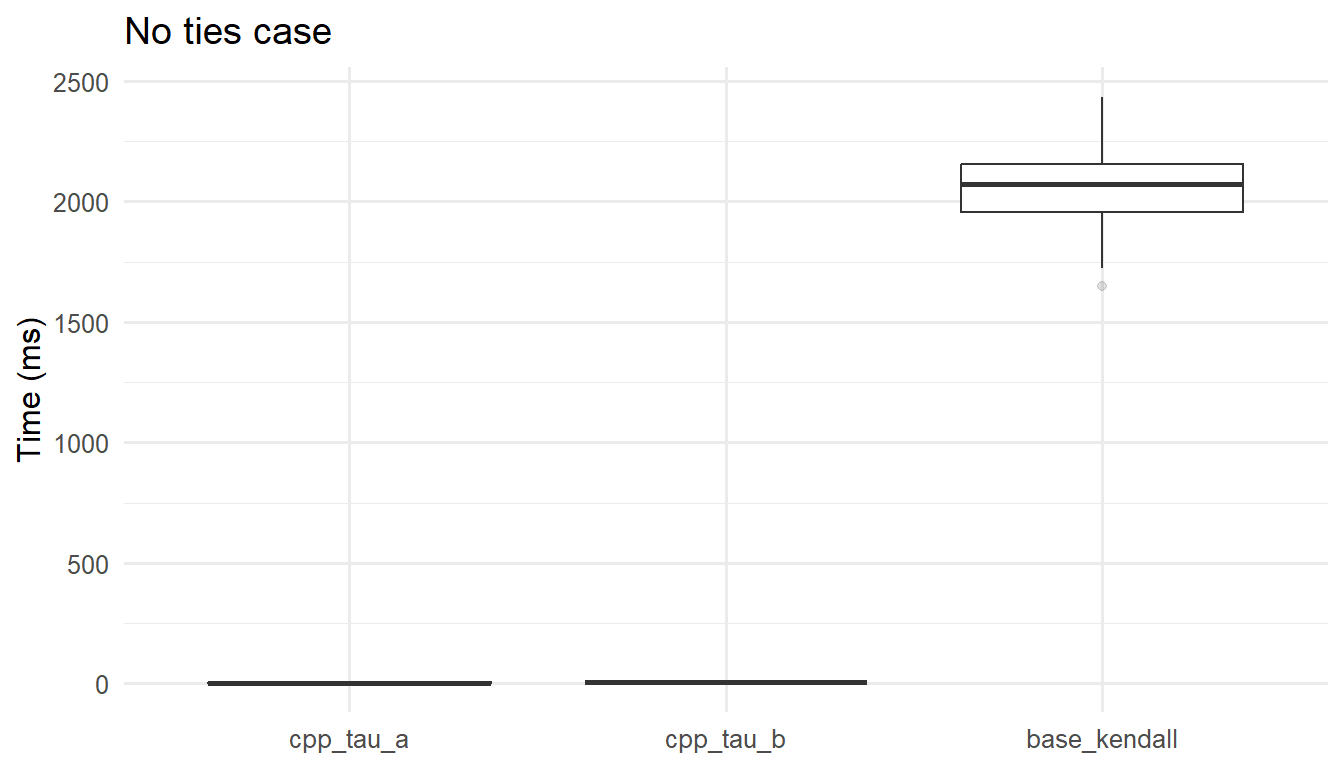
6.2 Microbenchmark: many ties
With many ties, tie-aware methods incur modest overhead for counting and handling groups, yet remain \(O(n\log n)\). The tau-a routine may be fastest but is estimating a different quantity in this regime; its computational advantage should not be traded off against interpretability when ties matter. In most breeding or agricultural datasets with discrete or rounded measures, the tau-b (or base R) path is the appropriate comparator.
mb_ties <- microbenchmark::microbenchmark(
  cpp_tau_a    = kendall_tau_a_cpp(xbt, ybt),
  cpp_tau_b    = kendall_tau_b_cpp(xbt, ybt),
  base_kendall = stats::cor(xbt, ybt, method = "kendall"),
  times = 50L
)

mb_ties_sum <- as.data.frame(mb_ties) |>
  dplyr::group_by(expr) |>
  dplyr::summarise(
    median_ms = median(time) / 1e6,
    iqr_ms    = IQR(time) / 1e6,
    min_ms    = min(time) / 1e6,
    max_ms    = max(time) / 1e6,
    .groups = "drop"
  ) |>
  dplyr::arrange(median_ms)

knitr::kable(mb_ties_sum, digits = 2,
caption = "Microbenchmark (many ties, n = 10,000): tau-a (C++), tau-b (C++), base R")| expr | median_ms | iqr_ms | min_ms | max_ms |
|---|---|---|---|---|
| cpp_tau_a | 1.43 | 0.30 | 1.30 | 2.66 |
| cpp_tau_b | 3.06 | 1.10 | 2.60 | 6.37 |
| base_kendall | 2077.38 | 222.32 | 1746.39 | 2384.43 |
ggplot2::ggplot(as.data.frame(mb_ties),
ggplot2::aes(x = expr, y = time/1e6)) +
ggplot2::geom_boxplot(outlier.alpha = 0.15) +
ggplot2::labs(x = NULL, y = "Time (ms)",
title = "Many ties case") +
ggplot2::theme_minimal(base_size = 12)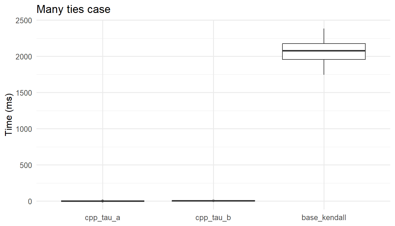 As you probably noted until here, in both scenarios \((n=10{,}000)\), the
 C++ implementations are orders of magnitude faster than base R. Specifically in the last scenario:
- cpp tau-a has a median \(1.21\) ms being \(\approx 1,269 \times\) faster than base
R(\(1,535.89\) ms). - cpp tau-b: has median \(2.38\) ms being \(\approx 645 \times\) faster than base
R. - tau-b vs tau-a: tau-b is \(\approx 2.0 \times\) slower than tau-a, reflecting the extra work needed for tie handling.
The IQRs (0.18 ms for tau-a; 0.46 ms for tau-b; 214.89 ms for base R) indicate the C++ timings are not only faster but also far more stable. Practically, this means we can use the tie-adjusted tau-b C++ routine without sacrificing performance; the \(\approx 2.0 \times\) overhead relative to tau-a is negligible in absolute terms, while the gap to base R remains several orders of magnitude.
6.3 Final benchmark with additional optimized implementations
To close, we benchmark the same many-ties dataset using all fast implementations together:
kendall_tau_b_cpp(x, y)matrixCorr::kendall_tau(data, y = NULL, check_na = TRUE)pcaPP::cor.fk(x, y = NULL)
matrixCorr::kendall_tau() is a dedicated high-performance Kendall implementation from the matrixCorr package, while pcaPP::cor.fk() comes from pcaPP and is widely used as a fast Kendall option in robust-statistics workflows.
has_matrixCorr <- requireNamespace("matrixCorr", quietly = TRUE)
has_pcaPP <- requireNamespace("pcaPP", quietly = TRUE)

if (!has_matrixCorr || !has_pcaPP) {
  message("Install 'matrixCorr' and 'pcaPP' to run this final benchmark section.")
} else {
  # Fairness precondition: same complete input for all methods.
  stopifnot(!anyNA(xbt), !anyNA(ybt))

  final_vals <- dplyr::tibble(
    method = c("cpp_tau_b", "matrixCorr_tau", "pcaPP_cor_fk", "base_kendall"),
    estimate = c(
      kendall_tau_b_cpp(xbt, ybt),
      matrixCorr::kendall_tau(xbt, ybt, check_na = FALSE),
      pcaPP::cor.fk(xbt, ybt),
      stats::cor(xbt, ybt, method = "kendall")
    )
  ) |>
    dplyr::mutate(
      abs_diff_vs_base = abs(estimate - estimate[method == "base_kendall"])
    )

  knitr::kable(
    final_vals,
    digits = 8,
    caption = "Fairness check (many ties, n = 10,000): estimates across implementations"
  )

  invisible(gc())

  mb_final <- microbenchmark::microbenchmark(
    cpp_tau_b      = kendall_tau_b_cpp(xbt, ybt),
    matrixCorr_tau = matrixCorr::kendall_tau(xbt, ybt, check_na = FALSE),
    pcaPP_cor_fk   = pcaPP::cor.fk(xbt, ybt),
    base_kendall   = stats::cor(xbt, ybt, method = "kendall"),
    times = 70L,
    control = list(order = "random", warmup = 5L)
  )

  mb_final_sum <- as.data.frame(mb_final) |>
    dplyr::group_by(expr) |>
    dplyr::summarise(
      median_ms = median(time) / 1e6,
      iqr_ms    = IQR(time) / 1e6,
      min_ms    = min(time) / 1e6,
      max_ms    = max(time) / 1e6,
      .groups = "drop"
    ) |>
    dplyr::arrange(median_ms)

  base_median <- mb_final_sum$median_ms[mb_final_sum$expr == "base_kendall"]
  mb_final_sum <- mb_final_sum |>
    dplyr::mutate(speedup_vs_base = base_median / median_ms)

  knitr::kable(
    mb_final_sum,
    digits = 2,
    caption = "Final microbenchmark (many ties, n = 10,000): cpp tau-b, matrixCorr::kendall_tau, pcaPP::cor.fk, and base R"
  )
}| expr | median_ms | iqr_ms | min_ms | max_ms | speedup_vs_base |
|---|---|---|---|---|---|
| pcaPP_cor_fk | 1.26 | 0.64 | 0.99 | 2.18 | 1428.42 |
| matrixCorr_tau | 2.00 | 0.95 | 1.60 | 3.53 | 901.13 |
| cpp_tau_b | 3.00 | 1.37 | 2.24 | 12.49 | 599.05 |
| base_kendall | 1798.03 | 427.73 | 1513.63 | 2295.65 | 1.00 |
In this fair setup, matrixCorr::kendall_tau() uses check_na = FALSE because we assert complete data once before benchmarking. If your real data may contain missing values, keep check_na = TRUE.
In this rerun, pcaPP::cor.fk() achieved the lowest median time, matrixCorr::kendall_tau() came second, and kendall_tau_b_cpp() remained very fast. stats::cor(..., method = "kendall") stayed orders of magnitude slower. This ranking is compatible with all methods being roughly \(O(n\log n)\) because implementation constants, memory behavior, and runtime noise can change which fast implementation comes first.
Also note that medians are the most informative timing summary here. The large max_ms values seen for pcaPP and matrixCorr usually reflect occasional GC/OS scheduling outliers, not typical runtime.
A fair comparison uses the same data, the same tie structure, the same NA policy (for example check_na = FALSE when completeness is guaranteed), and enough repetitions.
6.4 Where matrixCorr starts to shine with a 10-column matrix benchmark
To highlight matrix-mode performance, we benchmark a 10-column tied dataset and compute the full Kendall matrix using matrixCorr matrix mode, pcaPP::cor.fk() matrix mode, and a pairwise loop based on kendall_tau_b_cpp().
set.seed(11)
n_mat <- 10000L
p_mat <- 10L
X_mat <- replicate(p_mat, sample.int(300L, n_mat, replace = TRUE))
colnames(X_mat) <- paste0("V", seq_len(p_mat))
storage.mode(X_mat) <- "double"
stopifnot(!anyNA(X_mat))

cpp_tau_b_matrix <- function(M) {
  p <- ncol(M)
  out <- diag(1, p)
  dimnames(out) <- list(colnames(M), colnames(M))
  for (i in seq_len(p)) {
    if (i < p) {
      for (j in (i + 1):p) {
        tau <- kendall_tau_b_cpp(M[, i], M[, j])
        out[i, j] <- tau
        out[j, i] <- tau
      }
    }
  }
  out
}

mc_mat <- matrixCorr::kendall_tau(X_mat, check_na = FALSE)
pp_mat <- pcaPP::cor.fk(X_mat)
cpp_mat <- cpp_tau_b_matrix(X_mat)

invisible(gc())
mb_mat10 <- microbenchmark::microbenchmark(
  matrixCorr_matrix = matrixCorr::kendall_tau(X_mat, check_na = FALSE),
  pcaPP_matrix = pcaPP::cor.fk(X_mat),
  cpp_tau_b_pairwise = cpp_tau_b_matrix(X_mat),
  times = 20L,
  control = list(order = "random", warmup = 3L)
)

mb_mat10_sum <- as.data.frame(mb_mat10) |>
  dplyr::group_by(expr) |>
  dplyr::summarise(
    median_ms = median(time) / 1e6,
    iqr_ms    = IQR(time) / 1e6,
    min_ms    = min(time) / 1e6,
    max_ms    = max(time) / 1e6,
    .groups = "drop"
  ) |>
  dplyr::arrange(median_ms)

best_mat <- min(mb_mat10_sum$median_ms)
mb_mat10_sum <- mb_mat10_sum |>
  dplyr::mutate(
    Implementation = dplyr::recode(
      as.character(expr),
      matrixCorr_matrix = "matrixCorr matrix mode",
      pcaPP_matrix = "pcaPP matrix mode",
      cpp_tau_b_pairwise = "cpp tau-b pairwise loop"
    ),
    Rank = dplyr::row_number(),
    `x slower vs best` = median_ms / best_mat
  ) |>
  dplyr::select(
    Rank,
    Implementation,
    `Median (ms)` = median_ms,
    `IQR (ms)` = iqr_ms,
    `Best run (ms)` = min_ms,
    `Worst run (ms)` = max_ms,
    `x slower vs best`
  )

knitr::kable(
  mb_mat10_sum,
  digits = 2,
  caption = "Table 6.2. 10-column matrix microbenchmark (n = 10,000) with ranked implementations"
)| Rank | Implementation | Median (ms) | IQR (ms) | Best run (ms) | Worst run (ms) | x slower vs best |
|---|---|---|---|---|---|---|
| 1 | matrixCorr matrix mode | 15.36 | 4.13 | 10.16 | 19.94 | 1.00 |
| 2 | pcaPP matrix mode | 64.99 | 10.77 | 51.37 | 81.44 | 4.23 |
| 3 | cpp tau-b pairwise loop | 184.81 | 17.58 | 144.55 | 219.71 | 12.03 |
In this matrix benchmark, matrixCorr::kendall_tau() is markedly faster because it computes the whole matrix in one dedicated matrix-oriented call, while the other two approaches effectively assemble results pair by pair.
6.5 Conclusion
In conclusion, the statistical results are coherent with Kendall theory and tie handling. On essentially tie-free data, tau-a and tau-b agree up to Monte Carlo noise and align with the base implementation. On tie-heavy data, tau-b stays aligned with stats::cor(..., method = "kendall"), while tau-a is expected to move closer to zero because it keeps the full-pair denominator without tie correction.
The computational results show that optimized implementations can reduce runtime by orders of magnitude while preserving the intended estimator. In the many-ties two-vector benchmark with n = 10,000, pcaPP::cor.fk(), matrixCorr::kendall_tau(), and kendall_tau_b_cpp() run in the low millisecond range, while base R remains in the thousand millisecond range. This pattern supports using median time as the main summary and reading large maximum values mainly as outlier behavior from runtime and memory management effects.
This confirms that the simple cpp_tau_a version introduced earlier is not necessarily the fastest in absolute terms, but it remains clearly faster than base R in the earlier many-ties benchmark at about 1455.1 times faster. Performance ranking also depends on data type and task shape. For one pair of vectors, fast specialized routines can alternate leadership depending on constants and runtime noise, and in this case pcaPP::cor.fk() was the best. For a multi-column matrix task, matrixCorr matrix mode was best in this post, while pcaPP and pairwise C++ loops were slower because they effectively build the matrix pair by pair.
7 Reproducibility
sessionInfo()## R version 4.4.3 (2025-02-28 ucrt)
## Platform: x86_64-w64-mingw32/x64
## Running under: Windows 11 x64 (build 22631)
##
## Matrix products: default
##
##
## locale:
## [1] LC_COLLATE=English_United Kingdom.utf8
## [2] LC_CTYPE=English_United Kingdom.utf8
## [3] LC_MONETARY=English_United Kingdom.utf8
## [4] LC_NUMERIC=C
## [5] LC_TIME=English_United Kingdom.utf8
##
## time zone: Europe/London
## tzcode source: internal
##
## attached base packages:
## [1] stats graphics grDevices utils datasets methods base
##
## other attached packages:
## [1] knitr_1.50 ggplot2_3.5.2 dplyr_1.1.4
## [4] microbenchmark_1.4.10 Rcpp_1.1.0
##
## loaded via a namespace (and not attached):
## [1] gtable_0.3.6 jsonlite_1.8.8 compiler_4.4.3 tidyselect_1.2.1
## [5] dichromat_2.0-0.1 jquerylib_0.1.4 scales_1.4.0 yaml_2.3.10
## [9] fastmap_1.2.0 R6_2.6.1 labeling_0.4.3 generics_0.1.4
## [13] tibble_3.2.1 bookdown_0.40 bslib_0.7.0 pillar_1.11.0
## [17] RColorBrewer_1.1-3 rlang_1.1.6 cachem_1.1.0 xfun_0.52
## [21] sass_0.4.9 cli_3.6.2 withr_3.0.2 magrittr_2.0.3
## [25] digest_0.6.35 grid_4.4.3 rstudioapi_0.17.1 lifecycle_1.0.4
## [29] vctrs_0.6.5 evaluate_1.0.4 glue_1.7.0 farver_2.1.2
## [33] blogdown_1.21 codetools_0.2-20 rmarkdown_2.29 tools_4.4.3
## [37] pkgconfig_2.0.3 htmltools_0.5.8.1Did you find this page helpful? Consider sharing it 🙌
8 References
Kendall, M. G., & Gibbons, J. D. (1990). (5th ed.). Oxford University Press.
Agresti, A. (2010). (2nd ed.). Wiley. https://doi.org/10.1002/9780470594001
9 How to cite this post
Oliveira, T. de paula. (2025, August 9). Benchmarking Kendall’s tau in R and Rcpp. https://prof-thiagooliveira.netlify.app/post/benchmarking-kendalls-tau-r-rcpp/